Visualizing the Binomial Distribution (6.6)
TLDRThis video script delves into the binomial distribution, illustrating its formula and application with a coin flip example. It explains how varying the number of trials (n) and the probability of success (p) affects the distribution's shape, which can skew or become symmetrical. The script also covers how the binomial distribution approaches a normal distribution as n increases, and provides a guideline for when a normal approximation can be assumed. It concludes with the parameters of a binomial distribution, including mean, variance, and standard deviation.
Takeaways
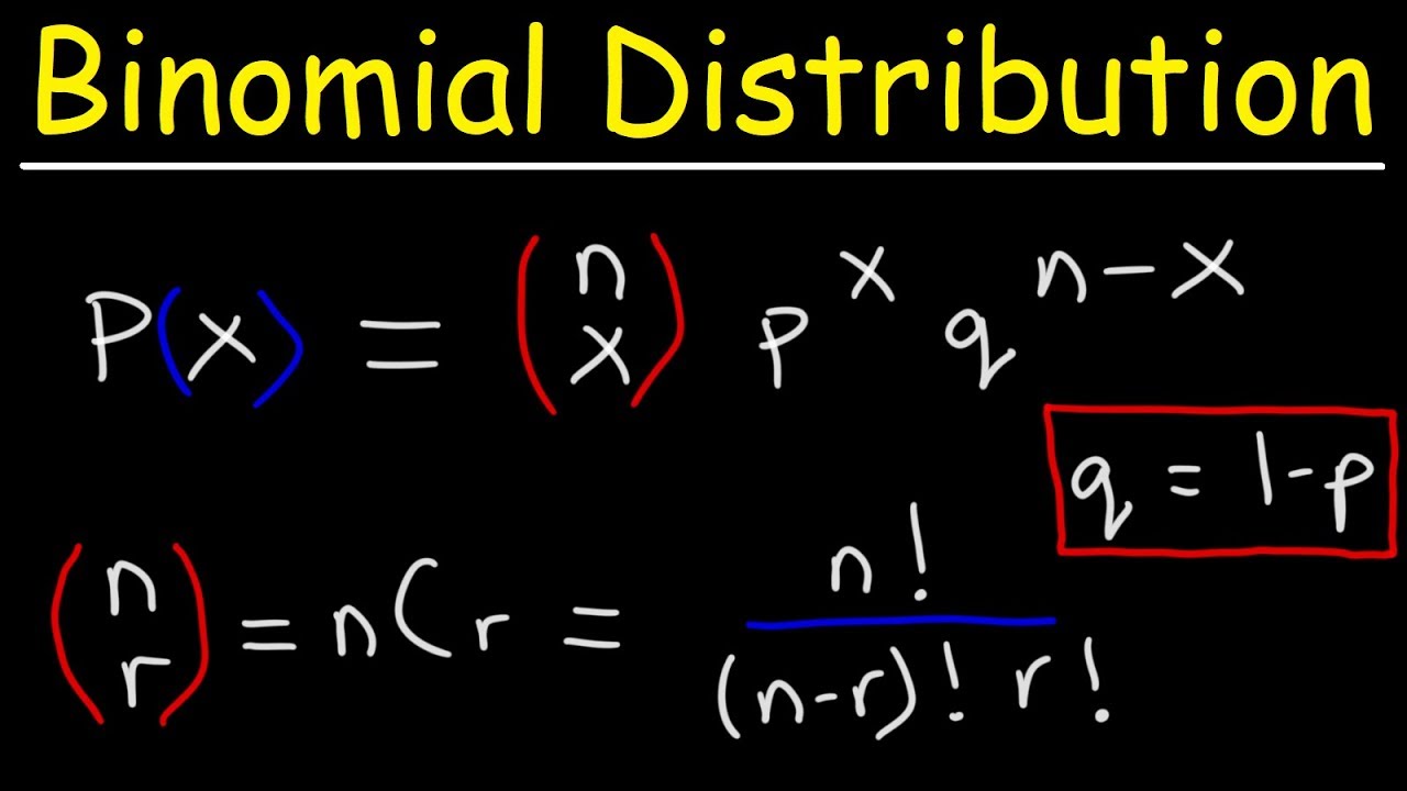
- 📘 The video covers the binomial distribution and reviews the binomial formula.
- 🪙 The formula calculates the probability of getting a certain number of successes in a set number of trials.
- 🔢 Example: Flipping a coin twice gives probabilities for 0, 1, or 2 successes.
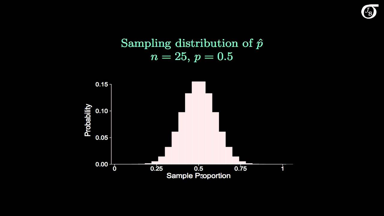
- 📊 The binomial distribution can be visualized with a bar chart showing probabilities for each number of successes.
- 🔄 Increasing the number of trials makes the binomial distribution resemble a normal distribution.
- 📈 The mean (μ) of a binomial distribution is n times p, and the variance is np(1-p).
- 🔄 The shape of the binomial distribution changes with the probability of success (p).
- ⚖️ A probability (p) of 0.5 gives a symmetrical distribution, while deviations from 0.5 cause skewness.
- 🔢 Larger values of n make skewed distributions approach normality.
- 📏 Rough guideline: A binomial distribution can approximate a normal distribution if np and n(1-p) are both ≥ 10.
Q & A
What is the binomial distribution?
-The binomial distribution is a discrete probability distribution that describes the number of successes in a fixed number of independent Bernoulli trials with the same probability of success.
What are the key components of the binomial formula?
-The key components of the binomial formula are k (number of successes), n (number of trials), and p (probability of success).
If you flip a coin twice, what is the maximum number of 'successes' you can get, and why?
-The maximum number of 'successes' you can get is 2, because you are only flipping the coin twice, and each flip can result in a success (heads).
What is the probability of getting heads when flipping a fair coin?
-The probability of getting heads when flipping a fair coin is 0.5, assuming it is a fair coin with two equally likely outcomes.
How does the binomial distribution visualize the probabilities of different numbers of successes?
-The binomial distribution can be visualized using a bar chart, where the x-axis represents the number of successes (k) and the y-axis represents the probability of success for each value of k.
What happens to the shape of the binomial distribution when the number of trials (n) increases?
-As the number of trials (n) increases, the binomial distribution begins to resemble a normal distribution, especially when n is large enough.
What are the parameters of a binomial distribution, and how are they calculated?
-The parameters of a binomial distribution are the mean (μ = np), variance (np(1-p)), and standard deviation (σ = √(np(1-p))).
How does the value of p affect the shape of the binomial distribution?
-The value of p affects the shape of the binomial distribution by causing it to be skewed. If p is less than 0.5, the distribution is skewed to the right; if p is greater than 0.5, it is skewed to the left. A p value of 0.5 results in a symmetrical distribution.
What is the mean of a binomial distribution, and how does it relate to the number of trials and the probability of success?
-The mean of a binomial distribution (μ) is equal to the number of trials (n) multiplied by the probability of success (p), indicating the expected number of successes in the trials.
Under what conditions can we assume a normal approximation for the binomial distribution?
-A normal approximation for the binomial distribution can be assumed if both np and n(1-p) are greater than or equal to 10, although some guidelines suggest using 5 instead of 10.
What is the relationship between the skewness of the binomial distribution and the value of p?
-The skewness of the binomial distribution is related to the value of p. A p value of 0.5 results in a symmetrical distribution, while values less than or greater than 0.5 cause the distribution to be skewed to the right or left, respectively.
Outlines
📊 Understanding the Binomial Distribution
This paragraph introduces the concept of the binomial distribution, starting with a review of the binomial formula. It explains the variables k (number of successes), n (number of trials), and p (probability of success) using the example of flipping a coin twice. The formula is applied to calculate the probabilities for each possible number of successes, resulting in 0.25, 0.50, and 0.25. The paragraph then discusses the visualization of these probabilities through a bar chart and explores how increasing the number of trials (n) affects the distribution's shape, approaching a normal distribution as n becomes larger. It also explains how the mean, variance, and standard deviation of a binomial distribution are calculated and how changing the value of p affects the distribution's symmetry, with deviations from 0.5 causing skewness.
🔍 Influence of n and p on Binomial Distribution
The second paragraph delves into the impact of the number of trials (n) and the probability of success (p) on the binomial distribution's shape. It explains that increasing n helps to normalize a skewed distribution, while symmetrical distributions require less of an increase in n to achieve normality. The paragraph provides a guideline for approximating a binomial distribution with a normal distribution, suggesting that n times p and n times (1-p) should both be greater than or equal to 10, although this threshold may vary. It concludes by summarizing the influence of p on the distribution's shape, noting that a p of 0.5 results in symmetry, while values above or below this lead to skewness in opposite directions. The mean, variance, and standard deviation formulas for a binomial distribution are reiterated, and the video ends with a call to support the creators and access additional study materials.
Mindmap
Keywords
💡Binomial Distribution
💡Binomial Formula
💡Successes (k)
💡Trials (n)
💡Probability of Success (p)
💡Bar Chart
💡Normal Distribution
💡Mean (μ)
💡Variance
💡Standard Deviation (σ)
💡Skewness
💡Normal Approximation
Highlights
Introduction to the binomial distribution and review of the binomial formula.
Explanation of the binomial formula components: k (number of successes), n (number of trials), and p (probability of success).
Illustration of calculating probabilities using the binomial formula with a coin flip example.
Visualization of binomial distribution through a bar chart for the coin flip scenario.
Demonstration of how increasing the number of trials (n) affects the shape of the binomial distribution.
Analysis of the mean, variance, and standard deviation of a binomial distribution.
Observation of the binomial distribution's resemblance to a normal distribution as n increases.
Impact of changing the value of p on the shape of the binomial distribution.
Explanation of the skewness in binomial distribution when p deviates from 0.5.
Example of a binomial distribution with p=0.1, showing high probability of fewer successes.
Contrasting example with p=0.8, illustrating a higher likelihood of more successes.
Discussion on the clustering of data around the mean in binomial distributions.
Guidelines for when a binomial distribution can be approximated by a normal distribution.
Importance of n and p values in achieving a normal approximation of the binomial distribution.
Recap of the influence of p on the skewness and symmetry of the binomial distribution.
Summary of the mean, variance, and standard deviation formulas for a binomial distribution.
Encouragement to support the creators on Patreon and visit their website for additional resources.
Transcripts
Browse More Related Video

The Sampling Distribution of the Sample Proportion

Finding The Probability of a Binomial Distribution Plus Mean & Standard Deviation

Math 119 Chapter 5 part 2

Types Of Distribution In Statistics | Probability Distribution Explained | Statistics | Simplilearn

Binomial Distribution EXPLAINED in UNDER 15 MINUTES!

Elementary Statistics - Chapter 5 Binomial Distributions Part 2
5.0 / 5 (0 votes)
Thanks for rating: