Gaussian Elimination & Row Echelon Form
TLDRThis video tutorial demonstrates the process of using Gaussian elimination to solve a system of linear equations with three variables. It begins by converting the system into an augmented matrix and then systematically transforms it into row echelon form. Through a series of matrix row operations, the video shows how to achieve a diagonal of ones with zeros below, which simplifies the system for easier solution. The method is applied to two different systems of equations, with the second example showing how to solve the system without fully converting it to row echelon form. The final solutions are presented clearly, illustrating the effectiveness of Gaussian elimination for finding the values of the variables.
Takeaways
- 📌 Gaussian elimination is a method used to solve systems of linear equations with three variables.
- 🔢 The first step is to convert the system of equations into an augmented matrix, which includes the coefficients and constants.
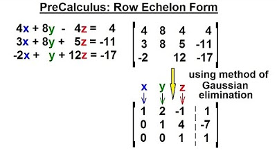
- 📐 The goal is to transform the augmented matrix into row echelon form, where the diagonal entries are 1s and the entries below are 0s.
- ➕ Row operations, such as adding or swapping rows, are used to manipulate the matrix into the desired form.
- 🔄 The process involves making the first non-zero entry of each row (leading entry) equal to 1, known as the pivot.
- 📈 After achieving row echelon form, back substitution can be used to solve for the variables x, y, and z.
- 🤔 The script provides a step-by-step example of solving a system of equations using Gaussian elimination and back substitution.
- 📝 The example demonstrates how to perform row operations to achieve the necessary form for solution and how to interpret the results.
- 🌟 The video emphasizes the importance of careful calculation and attention to detail when performing row operations.
- 🎯 The method can be applied to different systems of equations, as shown in the second example provided in the script.
- 📋 The script serves as a guide for those looking to understand and apply Gaussian elimination to solve systems of linear equations.
Q & A
What is the main topic of the video?
-The main topic of the video is using Gaussian elimination to solve a system of equations with three variables.
How many equations are given in the problem?
-There are three equations given in the problem.
What is the augmented matrix for the first set of equations?
-The augmented matrix for the first set of equations is: [ 1 1 -1 | -2 ] [ 2 -1 1 | 5 ] [-1 2 2 | 1 ]
What is the goal when converting the matrix into row echelon form?
-The goal when converting the matrix into row echelon form is to have a diagonal of ones and zeros below the diagonal.
What is the first row operation performed on the matrix?
-The first row operation performed is adding row one to row three.
How is the second row transformed to have a zero in the second column?
-The second row is transformed by multiplying row one by -2 and then adding it to row two.
What is the solution for the first set of equations after applying Gaussian elimination?
-The solution for the first set of equations is x = 1, y = -1, and z = 2.
What is the second set of equations given in the video?
-The second set of equations given are: 2X + y - Z = 1 3x + 2y + Z = 10 2x - y + 2z = 6
How is the second set of equations initially transformed?
-The second set of equations is initially transformed by converting it into an augmented matrix and then performing a series of row operations to make the leading coefficients zeros.
What is the solution for Z in the second set of equations?
-The solution for Z in the second set of equations is Z = 3.
What is the final solution for the second set of equations?
-The final solution for the second set of equations is x = 1, y = 2, and z = 3.
Outlines
🧮 Solving a System of Equations Using Gaussian Elimination
This video begins by introducing a problem involving a system of equations with three variables: x, y, and z. The equations are converted into an augmented matrix format. The tutorial demonstrates the process of converting the matrix into row echelon form through specific matrix row operations. The initial operations focus on making pivotal elements into ones and other elements in the column into zeros, starting with the transformation of the matrix by adding and modifying rows. Detailed step-by-step calculations are presented, showing the viewer how to systematically manipulate the matrix to achieve the desired form.
🔍 Completing the Gaussian Elimination Process
Continuing from the previous steps, this section deals with further manipulation of the matrix to solve for variables x, y, and z. It explains how to make specific matrix entries zero and then how to normalize rows to have leading ones. The tutorial progresses to convert the matrix entries back into a system of linear equations and then uses back-substitution to solve for z, y, and finally x. Detailed explanations and mathematical operations demonstrate converting matrix rows to simplified forms and then extracting and solving linear equations from these forms.
📉 Using Gaussian Elimination for Another System
This segment introduces a new set of equations and converts them into an augmented matrix, focusing on making strategic zeros to simplify the matrix without fully converting it to row echelon form. Specific operations include subtracting and adding rows, and adjusting matrix entries through multiplication to make certain elements zero. The resulting simplified matrix allows for solving the equations directly for z, y, and x, showcasing a practical application of Gaussian elimination to derive solutions efficiently.
🧐 Extracting Solutions from a Simplified Matrix
In this final section, the simplified matrix setup from the previous paragraph is used to directly solve for z, y, and x. The video demonstrates how to derive z from the simplest equation and then use its value to solve for y in the next simplest equation. Finally, x is derived by substituting the values of y and z into the first equation. The section efficiently illustrates how Gaussian elimination, even without full conversion to row echelon form, can be effectively used to quickly find solutions to a system of equations.
Mindmap
Keywords
💡Gaussian Elimination
💡Augmented Matrix
💡Row Echelon Form
💡Back Substitution
💡Row Operations
💡Pivot
💡Linear Equations
💡Variables
💡Matrix
💡Systems of Equations
💡Solving Equations
Highlights
Introduction to using Gaussian elimination to solve a system of equations with three variables. (Start time: 0s)
Formulation of the initial system of equations with three variables. (Start time: 10s)
Conversion of the system to an augmented matrix. (Start time: 20s)
Explanation of the goal to transform the matrix into row echelon form. (Start time: 30s)
First row operation: adding row one to row three. (Start time: 40s)
Second row operation: converting the 2 into a 0 by applying changes to row two. (Start time: 50s)
Third row operation: adding rows two and three to eliminate the number in the third row, second column. (Start time: 1m 10s)
Conversion of the matrix into row echelon form with a diagonal of ones. (Start time: 1m 30s)
Solution extraction from the row echelon form: identifying the value of Z. (Start time: 1m 50s)
Back substitution to find the values of Y and X. (Start time: 2m 10s)
Final solution of the system of equations: X = 1, Y = -1, Z = 2. (Start time: 2m 30s)
Introduction to another example with a different system of equations. (Start time: 2m 50s)
Conversion of the new system into an augmented matrix. (Start time: 3m 10s)
Performing Gaussian elimination to achieve three zeros in the key positions. (Start time: 3m 30s)
Solving the system without full conversion to row echelon form: identifying the value of Z. (Start time: 3m 50s)
Continued back substitution to find the values of Y and X for the second example. (Start time: 4m 10s)
Final solution of the second system of equations: X = 1, Y = 2, Z = 3. (Start time: 4m 30s)
Transcripts
Browse More Related Video

PreCalculus - Matrices & Matrix Applications (5 of 33) Method of Gaussian Elimination: Example

PreCalculus - Matrices & Matrix Applications (3 of 33) Row Echelon Form

Algebra 55 - Gauss-Jordan Elimination

Gaussian Elimination With 4 Variables Using Elementary Row Operations With Matrices

Solving System of Linear Equations: Gaussian Elimination

PreCalculus - Matrices & Matrix Applications (7 of 33) Method of Gaussian Elimination: 3x3 Matrix*
5.0 / 5 (0 votes)
Thanks for rating: