Avon High School - AP Calculus BC - Topic 10.11 - Example 1
TLDRThis video script introduces the concept of infinite series and their significance in AP Calculus BC, particularly for understanding approximations of functions. It delves into the history of mathematical approximations and sets the stage for exploring quadratic approximations. The video outlines the process of linear approximation and its limitations, leading to the introduction of quadratic approximation as a more accurate method. The script provides a detailed explanation of constructing a quadratic approximation, using the natural logarithm function as an example. It concludes with a practical application, demonstrating how to estimate the natural log of 1.05 using both linear and quadratic approximations, and highlights the improved accuracy of higher-degree polynomials in modeling functions.
Takeaways
- 📚 The video introduces foundational concepts for understanding infinite series in AP Calculus BC, particularly in relation to the end of the course.
- 🔍 The historical context of mathematicians approximating complex functions without modern computational tools is discussed, highlighting the importance of the techniques to be covered.
- 📈 The concept of linear approximation is reviewed from Topic 4.6, emphasizing its limitations when dealing with functions with high curvature.
- 📊 A new approximation method, quadratic approximation, is introduced to overcome the limitations of linear approximation by adding a second-degree term to the polynomial model.
- 🔧 The process of creating a quadratic approximation involves finding the function's value, slope, and concavity at a specific point c, and ensuring the polynomial agrees with these properties.
- 👓 The video provides a detailed walkthrough of constructing a quadratic approximation for the natural logarithm function, ln(x), at x=1.
- 🧮 The linear and quadratic approximations for ln(x) are used to estimate the value of ln(1.05), demonstrating the practical application of the concepts.
- 📊 Graphing the natural logarithm function, its linear approximation, and its quadratic approximation visually illustrates the improved fit of the quadratic model over a wider range.
- 🤔 The accuracy of the quadratic approximation is compared to the actual value of ln(1.05), showing a close approximation with a high degree polynomial.
- 🎯 The video concludes with the introduction of the term 'Taylor Polynomial' as the method for approximating functions using higher degree polynomials.
- 🚀 The content is part of a series of videos aimed at deepening understanding of calculus concepts, with more to come for AP Calculus BC students.
Q & A
What is the main focus of this video for AP Calc BC students?
-The main focus of this video is to introduce the concept of infinite series and its importance in the later parts of the AP Calc BC course, specifically in relation to quadratic approximations.
How did mathematicians approximately compute complex functions without graphing calculators centuries ago?
-Mathematicians used techniques similar to those used by calculators today, relying on methods that could be performed with pencil and paper to achieve accurate results for complex functions.
What is linear approximation in the context of calculus?
-Linear approximation is a process where a curve is approximated by finding a tangent line at a specific point on the curve, which can be used to determine information about the curve's behavior near that point.
What are the two main properties of a first-degree polynomial used in linear approximation?
-The two main properties are: 1) it matches the function in value at the specific point (c), and 2) its slope matches the slope of the function at that point (x=c).
Why is a quadratic approximation sometimes preferred over a linear approximation?
-A quadratic approximation is preferred when the graph has a significant degree of curvature, as linear approximations may not provide accurate results in such cases.
What is the general form of a quadratic approximating polynomial?
-The general form of a quadratic approximating polynomial is p_sub_2(x) = f(c) + f'(c)(x - c) + a(x - c)^2, where a is a constant that needs to be determined.
What are the three conditions that a quadratic approximation must satisfy to be a good model for a function near a point c?
-The three conditions are: 1) the approximation must agree with the function in value at c, 2) its slope must match the function's slope at c, and 3) its concavity (second derivative) must match the function's concavity at c.
How is the constant 'a' in the quadratic approximation determined?
-The constant 'a' is determined by setting it equal to f''(c)/2, where f''(c) is the second derivative of the function at the point c.
What function is used as an example to demonstrate linear and quadratic approximations in the video?
-The natural logarithm function, ln(x), is used as an example to demonstrate both linear and quadratic approximations.
How accurate is the quadratic approximation in estimating the natural log of 1.05?
-The quadratic approximation is quite accurate, with an estimated value of 0.04875, which is only about 1 in 100,000 away from the actual value of 0.04879.
What is the significance of the Taylor polynomial introduced in the video?
-The Taylor polynomial is a high-degree polynomial that provides an increasingly accurate approximation of a function by including more terms based on the function's derivatives at a specific point.
Outlines
📚 Introduction to Infinite Series and Approximations
The paragraph introduces the concept of infinite series and their significance in the Advanced Placement Calculus BC course, particularly in the context of the final unit. It emphasizes the historical challenge of computing complex functions without modern tools and sets the stage for learning foundational information that will lead into examples over topics 10 and 11. The discussion begins with the importance of understanding how mathematicians approximated functions in the past, hinting at the relevance of these techniques to modern calculator computations.
📈 Linear vs. Quadratic Approximations
This section delves into the difference between linear and quadratic approximations. It starts by revisiting the concept of linear approximation from a previous topic, explaining how it involves finding a tangent line to a curve at a specific point. The paragraph then introduces the quadratic approximation, which involves adding a new term to the linear polynomial to better model the curve, especially when there is significant curvature. The process of determining the coefficients for the quadratic approximation is outlined, emphasizing the need for the approximation to match the function in value, slope, and concavity at a given point.
🧮 Example: Linear and Quadratic Approximations of ln(x)
The paragraph presents a specific example of approximating the natural logarithm function (ln(x)) using both linear and quadratic approximations. It details the steps to find the linear approximation at x=1 and then extends this to create a quadratic approximation. The process involves calculating the first and second derivatives of ln(x) and using these to construct the approximating polynomials. The example illustrates the methodology for applying the concepts discussed in the previous paragraphs.
📊 Graphing and Estimating with Approximations
This part of the script discusses the practical application of the linear and quadratic approximations by graphing them alongside the actual function, ln(x). It explains how to use the approximations to estimate the value of ln(1.05) and compares the results with the actual value obtained from a calculator. The paragraph highlights the improved accuracy of the quadratic approximation over the linear one, especially when moving away from the point of tangency, and visually demonstrates this improvement through graphing on a calculator.
🎓 Taylor Polynomial Introduction and Conclusion
The final paragraph wraps up the discussion by introducing the concept of Taylor polynomials, which are a series of approximations that can be used to closely replicate a function. It reflects on the accuracy achieved through higher-degree polynomials and the importance of these approximations in understanding complex mathematical functions. The script ends with a call to action for viewers to subscribe for more content and a teaser for upcoming videos.
Mindmap
Keywords
💡AP Calc BC
💡Infinite Series
💡Quadratic Approximation
💡Linear Approximation
💡Point-Slope Formula
💡Derivative
💡Tangent Line
💡Natural Logarithm
💡Taylor Polynomial
💡Engineering Feats
Highlights
Introduction to the concept of infinite series and their importance in the study of calculus.
Foundational information on how to approximate functions using polynomials, which is crucial for understanding calculus BC.
Historical context of mathematicians computing complex functions without modern tools, showcasing the evolution of computational techniques.
Explanation of linear approximation using the point-slope formula, setting the stage for more advanced approximation methods.
Transition from linear to quadratic approximation, adding a new term to improve the model's accuracy.
Derivation of the quadratic approximation polynomial, including the conditions it must satisfy to accurately model the function.
Detailed process of finding the value of 'a' in the quadratic approximation to ensure the model's concavity matches the original function.
Example of approximating the natural log function using both linear and quadratic approximations, demonstrating the practical application of these concepts.
Comparison of the accuracy of linear and quadratic approximations through the estimation of ln(1.05), highlighting the benefits of higher-degree polynomials.
Introduction to Taylor polynomials as a method of approximating functions, providing a glimpse into advanced calculus topics.
Discussion on the importance of precision in engineering feats of the past, linking historical achievements with modern mathematical techniques.
Explanation of how the derivative of a function is used in creating approximation models, emphasizing the role of calculus in the process.
Illustration of how the slope of the approximating polynomial must match the slope of the original function at the point of approximation.
Demonstration of the mathematical process of taking derivatives and evaluating them at specific points to build the approximation model.
Visual representation of the natural log function and its approximations through graphing, showing the effectiveness of quadratic over linear models.
Mistake correction during the live explanation, emphasizing the importance of accuracy in mathematical communication.
Conclusion that higher-degree polynomials, like the Taylor polynomial introduced, provide more accurate representations of functions.
Transcripts
Browse More Related Video
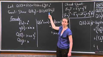
Quadratic Approximation of a Product | MIT 18.01SC Single Variable Calculus, Fall 2010
What do quadratic approximations look like
Avon High School - AP Calculus BC - Topic 10.11 - Example 2

Taylor Polynomials Day 1
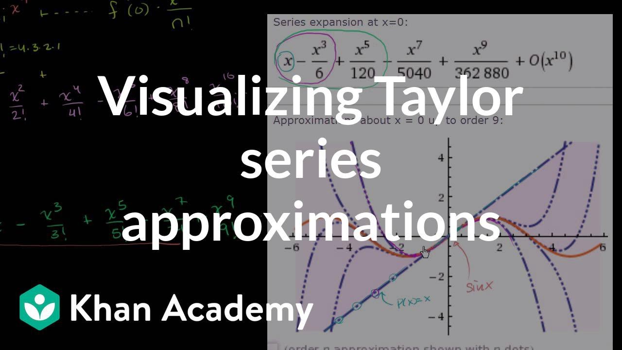
Visualizing Taylor series approximations | Series | AP Calculus BC | Khan Academy
Quadratic Approximation | MIT 18.01SC Single Variable Calculus, Fall 2010
5.0 / 5 (0 votes)
Thanks for rating: