Numerical Integration With Trapezoidal and Simpson's Rule

Professor Leonard

15 May 201427:07

EducationalLearning

32 Likes 10 Comments

TLDRThis video script delves into the concept of numerical integration, focusing on the trapezoidal rule and Simpson's rule as methods to approximate definite integrals when analytical solutions are infeasible. The instructor guides viewers through the process of applying these rules, providing step-by-step examples to clarify the calculations. The trapezoidal rule is explained first, followed by Simpson's rule, which requires an even number of intervals. The script emphasizes the importance of these techniques in approximating complex integrals and illustrates their practicality with examples, highlighting the accuracy achievable with a finite number of terms.

Takeaways

📚 Numerical integration is a method used to approximate definite integrals that cannot be solved analytically.
📉 Two common numerical integration techniques are the trapezoidal rule and Simpson's rule, both providing approximations for integrals.
🔍 The trapezoidal rule involves breaking the area under the curve into trapezoids and summing their areas to approximate the integral.
📐 The formula for the trapezoidal rule is given by "Δx × (f(x_0)/2 + 2 ∑ f(x_i) + f(x_n))", where "Δx" is the width of each trapezoid.
📝 In the trapezoidal rule, "Δx" is calculated as "(b - a) / n", with "n" being the number of trapezoids and "a" and "b" the bounds of integration.
📈 Simpson's rule is similar to the trapezoidal rule but uses a different weighting for the function values at each interval, resulting in a more accurate approximation.
🔢 Simpson's rule formula alternates between multiplying function values by 4 and 2, ending with a single function value without a multiplier, and requires "n" to be even.
📌 Both methods require selecting a finite number of intervals (or 'terms'), as taking the limit as "n" approaches infinity would result in the actual integral rather than an approximation.
🤔 The script provides an example of using the trapezoidal rule to approximate the integral of "1/x" from 1 to 2 using 10 intervals, illustrating the process step-by-step.
📊 The accuracy of numerical integration methods can be improved by increasing the number of intervals, resulting in smaller and more precise approximations of the area under the curve.
🔎 The script also compares the numerical approximations to the actual integrals when possible, demonstrating the closeness of the approximations to the true values.

Q & A

What is numerical integration and why is it used?
-Numerical integration is a method used to approximate definite integrals when an analytical solution is not available or is too complex to compute. It allows us to estimate the area under a curve by using numerical techniques when the integral cannot be solved exactly.
What are the two main numerical integration methods discussed in the script?
-The two main numerical integration methods discussed are the Trapezoidal Rule and Simpson's Rule. Both methods provide different ways to approximate the value of a definite integral.
How does the Trapezoidal Rule work?
-The Trapezoidal Rule works by dividing the area under the curve into trapezoids and summing their areas. It approximates the integral by taking the average of the function values at the endpoints of each subinterval, multiplying by 2 for all but the first and last terms, and adding the function value at the first and last points.
What is the formula for the Trapezoidal Rule?
-The formula for the Trapezoidal Rule is given by "Integral ≈ (Δx / 2) [f(x0) + 2f(x1) + 2f(x2) + ... + 2f(xn-1) + f(xn)]", where "Δx" is the width of each subinterval, and "xi" are the points within the interval.
How is the value of Δx calculated in the Trapezoidal Rule?
-In the Trapezoidal Rule, Δx is calculated as the total length of the interval (b - a) divided by the number of subintervals (N), where b and a are the bounds of integration.
What is Simpson's Rule and how does it differ from the Trapezoidal Rule?
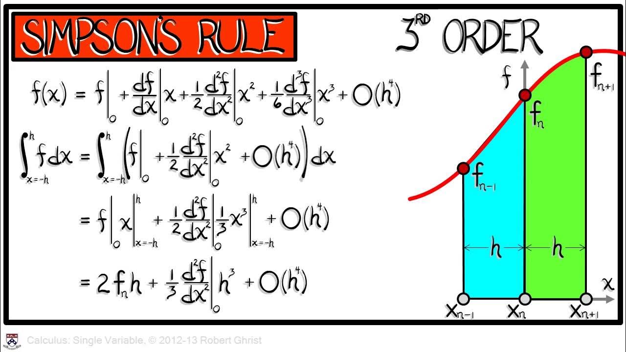
-Simpson's Rule is another method for approximating definite integrals. It differs from the Trapezoidal Rule by using a combination of rectangles and parabolas to approximate the area under the curve. The formula alternates between multiplying the function values by 4 and 2, and it requires an even number of subintervals.
What is the formula for Simpson's Rule?
-The formula for Simpson's Rule is "Integral ≈ (Δx / 3) [f(x0) + 4f(x1) + 2f(x2) + 4f(x3) + ... + f(xn)]", where the pattern of coefficients is 4, 2 repeated, and the last term has no coefficient.
Why does Simpson's Rule require an even number of subintervals?
-Simpson's Rule requires an even number of subintervals because the method relies on the parabolic shape that is formed between every three consecutive points. An even number of intervals ensures that this pattern can be consistently applied across the entire interval.
How can the accuracy of numerical integration methods be improved?
-The accuracy of numerical integration methods can be improved by increasing the number of subintervals (N). More subintervals result in smaller trapezoids or parabolas, which leads to a closer approximation of the actual area under the curve.
What is an example of a function that might be difficult to integrate analytically, as mentioned in the script?
-One example given in the script is the integral of 1/x, which is a natural logarithm function. This integral is not covered in early calculus courses and can be approximated using numerical integration methods.
How does the script demonstrate the application of the Trapezoidal Rule and Simpson's Rule?
-The script demonstrates the application of the Trapezoidal Rule and Simpson's Rule by walking through the process of approximating the integral of 1/x from 1 to 2 using the Trapezoidal Rule with N=10, and the integral of 1/√(x+1) from 0 to 2 using Simpson's Rule with N=6.

Outlines

00:00

📚 Introduction to Numerical Integration

This paragraph introduces the concept of numerical integration as a method to approximate definite integrals that cannot be solved analytically. It discusses two primary techniques: the trapezoidal rule and Simpson's rule. The speaker emphasizes that these methods are particularly useful for integrals not covered in standard calculus courses and provides a brief overview of how these rules function to give an approximation of the integral's value.

05:00

📐 The Trapezoidal Rule Explained

The speaker delves into the specifics of the trapezoidal rule, detailing its formula and how it is applied to approximate integrals. The explanation includes the calculation of 'Delta X' and the iterative process of summing function values at various intervals. An example is given to demonstrate the application of the trapezoidal rule using a function 1/x integrated from 1 to 2 with N=10, illustrating the step-by-step process and the resulting approximation.

10:03

🔍 Example Calculation with the Trapezoidal Rule

Building on the previous explanation, this paragraph walks through the actual calculation process of the trapezoidal rule using the example provided. It explains how to determine the values of 'X sub i' and how to plug these into the function to be integrated. The paragraph also compares the numerical approximation with the actual integral's result, showing the closeness of the approximation and discussing how increasing the number of terms can improve accuracy.

15:03

📉 Transition to Simpson's Rule

The speaker shifts focus to Simpson's rule, highlighting its similarities and differences with the trapezoidal rule. It outlines the formula for Simpson's rule, emphasizing the need for an even number of intervals (N) and the alternating pattern of coefficients in the rule. The paragraph sets the stage for an example calculation using Simpson's rule, aiming to show how it can also be used to approximate integrals effectively.

20:05

📊 Applying Simpson's Rule with an Example

This paragraph provides a step-by-step guide on how to apply Simpson's rule using the function 1/√x + 1 integrated from 0 to 2 with N=6. It explains the calculation of 'Delta X' and the iterative process of determining the 'X sub i' values. The speaker then demonstrates the application of the formula, alternating between multiplying by 4 and 2, and concludes with the final term without a coefficient. The paragraph aims to show the ease of using Simpson's rule for approximation.

25:56

🔢 Comparing Numerical Approximations with Actual Integrals

The final paragraph wraps up the discussion by comparing the numerical approximations obtained from the trapezoidal and Simpson's rules with the actual integrals. It provides a brief analysis of the results, showing how close the approximations are to the actual values. The speaker encourages the audience to verify the calculations and understand the process, emphasizing the effectiveness of these numerical methods for approximating integrals that cannot be solved analytically.

Mindmap

Keywords

💡Numerical Integration

Numerical integration is a set of algorithms for calculating the integral of a function, especially when an analytical solution is difficult or impossible to obtain. In the context of the video, numerical integration is central to the theme as it allows for the approximation of definite integrals using methods like the trapezoidal rule and Simpson's rule, which are discussed as part of the content.

💡Trapezoidal Rule

The trapezoidal rule is a numerical integration technique that approximates the definite integral of a function by constructing a trapezoid whose area represents the integral's value. The script explains this concept by showing how to approximate the integral of 1/x from 1 to 2 using this rule, emphasizing its utility when analytical integration is not feasible.

💡Simpson's Rule

Simpson's rule is another method of numerical integration that provides a more accurate approximation than the trapezoidal rule by using parabolas instead of trapezoids. The script introduces this rule as an alternative to the trapezoidal rule, noting that it requires an even number of intervals and results in a more precise approximation of the integral.

💡Definite Integral

A definite integral is an integral that has a specific range, known as the bounds of integration. The video script discusses the process of approximating definite integrals using numerical methods, such as the trapezoidal and Simpson's rules, as a way to find their values when direct integration is not possible.

💡Approximation

Approximation in the context of the video refers to the process of estimating the value of an integral using numerical methods when exact solutions are not available. The script uses the terms 'approximate' and 'approximation' to describe the outcomes of applying the trapezoidal and Simpson's rules to integrals.

💡Delta X (Δx)

In the script, Δx (delta x) represents the width of the intervals used in the trapezoidal and Simpson's rules for dividing the area under the curve into smaller segments. It is calculated as the difference between the upper and lower bounds of the integral divided by the number of intervals (N), and it plays a crucial role in the approximation process.

💡Integral

An integral is a fundamental concept in calculus that represents the area under a curve between two points. The video script discusses the challenges of finding integrals for certain functions and introduces numerical integration as a method to approximate these areas when analytical solutions are not known.

💡Function Evaluation

Function evaluation in the script refers to the process of plugging in specific values (x sub i) into the function to be integrated. This is a necessary step in both the trapezoidal and Simpson's rules, where the function's value at different points is used to estimate the area under the curve.

💡Ln (Natural Logarithm)

The natural logarithm, denoted as 'Ln' in the script, is a mathematical function that is the inverse of the exponential function. It is mentioned in the context of the actual integral of 1/x, which is the natural logarithm of the upper bound of integration minus the natural logarithm of the lower bound.

💡Calculus

Calculus is a branch of mathematics that deals with rates of change and accumulation. The script references 'calculus 1' and 'calculus 2' to situate the discussion within the broader context of mathematical education, indicating that numerical integration is a topic that builds upon foundational calculus concepts.

Highlights

Introduction to numerical integration as a method to approximate definite integrals that lack a direct formula.

Explanation of the trapezoidal rule for numerical integration.

Description of the Simpson's rule as an alternative method for numerical integration.

The formula for the trapezoidal rule is presented, including the use of ΔX and function evaluations at various points.

Clarification that ΔX is calculated as (B - A) / N, where N is the number of intervals.

The importance of choosing an appropriate value for N to balance approximation accuracy and computational effort.

A step-by-step guide on how to apply the trapezoidal rule to a given integral.

An example of approximating the integral of 1/X from 1 to 2 using the trapezoidal rule with N=10.

The significance of the function's evaluation at specific points in the trapezoidal rule.

A comparison between the trapezoidal rule and the actual integral of 1/X to demonstrate approximation accuracy.

The concept of increasing the number of terms to improve the accuracy of numerical integration.

The formula for Simpson's rule is introduced, highlighting the difference in coefficients compared to the trapezoidal rule.

The requirement that N must be an even number for Simpson's rule to be applicable.

An example calculation using Simpson's rule to approximate an integral with N=6.

The demonstration of how Simpson's rule alternates between coefficients of 4 and 2, excluding the first and last terms.

A final comparison between the approximations made by the trapezoidal rule and Simpson's rule with the actual integral values to assess accuracy.

The conclusion emphasizing the utility of numerical integration methods when direct integration is not feasible.

Transcripts

Browse More Related Video

Numerical Integration - Trapezoidal Rule & Simpson's Rule

Calculus Chapter 5 Lecture 49 Numerical Integration II

Lec 25 | MIT 18.01 Single Variable Calculus, Fall 2007

Lec 24 | MIT 18.01 Single Variable Calculus, Fall 2007

Calculus AB Homework 6.2 Riemann and Trapezoidal Sums

Simpson's Rule & Numerical Integration

Related Tags

Numerical Integration Calculus Techniques Trapezoidal Rule Simpson's Rule Integral Approximation Math Education Complex Integrals Educational Content Math Tutorial Approximation Methods