Lec 25 | MIT 18.01 Single Variable Calculus, Fall 2007
TLDRIn this educational video, the professor discusses numerical methods, focusing on numerical integration techniques such as the trapezoidal rule and Simpson's Rule. He illustrates these concepts using the integral of 1/x from 1 to 2, highlighting Simpson's Rule's accuracy. The professor also delves into the computation of the constant √(π/2) using a clever slicing method and connects it to an important function in mathematics. The lecture concludes with a review of exam expectations, including calculating definite integrals, performing numerical approximations, and solving problems related to areas and volumes, with an emphasis on choosing the right method for each problem.
Takeaways
- 📚 The lecture discusses numerical methods, specifically focusing on numerical integration techniques such as the trapezoidal rule and Simpson's Rule.
- 🔍 The professor illustrates numerical integration with the simple integral of 1/x from 1 to 2, highlighting the difference between the exact answer (ln 2) and numerical approximations.
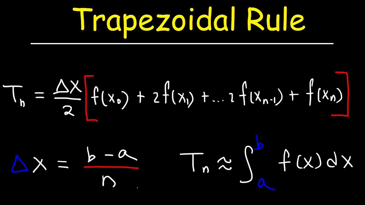
- 📈 The trapezoidal rule is shown to be a basic method for numerical integration, but it is not very accurate with only two intervals, resulting in a significant error.
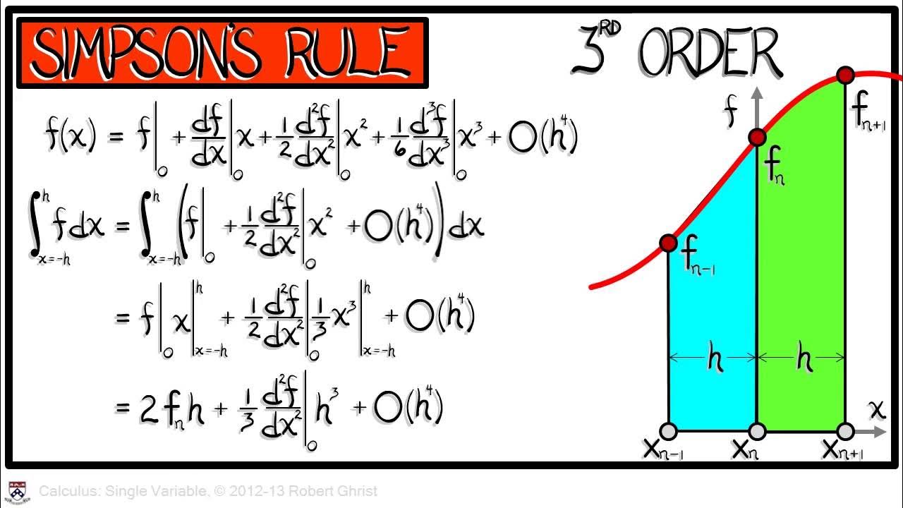
- 📉 Simpson's Rule is introduced as a more accurate method for numerical integration, with a formula that approximates the area under a curve more precisely than the trapezoidal rule.
- 📝 The professor emphasizes the importance of understanding the function being integrated, noting that Simpson's Rule works well for smooth functions but cautions about singularities near x=0.
- 📚 Simpson's Rule is derived from matching parabolas and is exact for all degree 2 polynomials, which contributes to its higher accuracy compared to other methods.
- 🧩 The professor connects the numerical methods to the calculation of a famous constant, the square root of pi/2, using the technique of slicing to find the area under a bell curve.
- 📐 The concept of volumes by slicing is introduced, where the volume of a solid is calculated by summing the areas of slices taken parallel to a certain plane.
- 📘 The script includes a detailed walkthrough of calculating the volume of a solid formed by rotating a function around an axis, leading to the discovery that V = Q^2 where V is the volume and Q is an area.
- 📝 The professor provides a review sheet and outlines the types of problems that will be on the exam, including definite integrals, numerical approximations, and calculating areas and volumes.
- ❓ The lecture concludes with a Q&A session where the professor addresses questions about Riemann sums, the choice between different numerical methods, and the determination of asymptotes.
Q & A
What is the primary focus of the lecture?
-The lecture focuses on numerical methods, particularly numerical integration, using examples like the trapezoidal rule and Simpson's rule.
What is the integral being evaluated in the lecture?
-The integral being evaluated is the integral from 1 to 2 of 1/x dx.
What is the exact value of the integral from 1 to 2 of 1/x dx?
-The exact value of the integral is ln(2).
How does the professor illustrate the accuracy of the numerical integration methods?
-The professor compares the numerical integration results to the exact value of ln(2) to demonstrate the accuracy of the methods.
What is the trapezoidal rule formula used in the lecture?
-The trapezoidal rule formula used is delta x (1/2 the first value + the second value + 1/2 the third value).
What result does the professor obtain using the trapezoidal rule for the integral from 1 to 2 of 1/x dx?
-Using the trapezoidal rule, the professor obtains approximately 0.96, which is far off from the exact value of ln(2).
What is Simpson's Rule formula as explained in the lecture?
-Simpson's Rule formula is (delta x / 3) (y_0 + 4 y_1 + y_2).
What result does the professor obtain using Simpson's Rule for the integral from 1 to 2 of 1/x dx?
-Using Simpson's Rule, the professor obtains approximately 0.69444, which is close to the exact value of ln(2).
Why is Simpson's Rule more accurate than the trapezoidal rule in this example?
-Simpson's Rule is more accurate because it matches the integral to a parabola, providing better approximation, especially for functions that fit well with quadratic functions.
What is the importance of ensuring the function is smooth for Simpson's Rule to work effectively?
-For Simpson's Rule to work effectively, the function must be smooth because it relies on the function's derivatives being well-behaved. If the function has singularities or is not smooth, the accuracy of Simpson's Rule can be compromised.
Outlines
📚 Introduction to Numerical Methods and MIT OpenCourseWare
The professor begins by acknowledging the support of the audience, which enables MIT OpenCourseWare to provide high-quality educational resources for free. Donations and additional materials can be found at ocw.mit.edu. The lecture then delves into numerical methods, specifically numerical integration, using the integral from 1 to 2 of dx/x as a simple example. The exact solution, ln(2), is contrasted with the numerical approximation obtained from a calculator, approximately 0.693147. The discussion highlights the accuracy achievable through numerical integration methods and the simplicity of the function 1/x in this context.
📉 Numerical Integration Techniques: Trapezoidal and Simpson's Rules
The professor compares two numerical integration methods: the trapezoidal rule and Simpson's Rule. The trapezoidal rule is demonstrated with a simple two-interval example, resulting in an approximation of 0.96, which is notably less accurate than the true value. Simpson's Rule is then introduced, claiming it to be more accurate, especially in this case, yielding an approximation of 0.69444, very close to the actual value of ln(2). The professor explains that Simpson's Rule works by matching a parabola to the curve, providing a more accurate estimation due to its higher-order validity. However, a caution is given regarding the limitations of Simpson's Rule when dealing with functions that have singularities or are not smooth, particularly near x equals 0.
📌 Simpson's Rule's Accuracy and its Application to Polynomials
The professor elaborates on Simpson's Rule's accuracy, noting that the error is approximately of the size of (delta x)^4, implying that increasing the number of intervals significantly improves accuracy. The rule's effectiveness is attributed to its derivation, which ensures exact answers for all parabolas and, coincidentally, for cubics as well. The professor emphasizes the importance of function smoothness and bounded derivatives for the rule to work effectively. A mnemonic device is suggested to remember the weights used in Simpson's Rule by checking it against the simplest case where the function f(x) equals 1.
🧩 Volume and Area Calculations Using Slicing Methods
The lecture shifts focus to the calculation of a mysterious constant, the square root of pi / 2, by using slicing methods. The professor reminds students of a previous computation involving the volume under the bell-shaped curve e^(-r^2) when rotated around an axis. The new problem involves calculating an area, which is approached by reimagining the volume calculation using slices. The professor hints at a trick where the volume V is found to be equal to the square of the area Q, leading to the conclusion that Q equals the square root of pi, once the volume V is known.
📐 Connecting Asymptotic Behavior with Slicing Methods
The professor connects the concept of asymptotic behavior to the slicing method used for calculating volumes and areas. The function discussed has an asymptote approaching the square root of pi / 2 as x goes to infinity. The professor illustrates the connection by showing that the area Q is twice the value of the function at infinity, thus confirming the earlier claim that the area under the curve from 0 to infinity is the square root of pi. The visualization of the function's graph and its asymptotic behavior is used to clarify the relationship between the volume and the area.
📈 Deriving the Formula for Volume by Slices
The professor introduces a three-dimensional perspective to visualize the slicing method for calculating volume. The x, y, and z axes are defined, with the z-axis representing the height of the slices formed by the rotation of the function e^(-r^2) around the z-axis. The professor explains the concept of a slice A(b) and how it relates to the volume calculation. The formula for the volume by slices is presented as the sum of the areas of the slices multiplied by their respective thicknesses, extending from negative infinity to positive infinity.
🔍 Calculating the Area of a Slice and Its Relation to the Total Volume
The professor focuses on calculating the area of a slice, A(b), by considering the function e^(-r^2) and expressing it in terms of b and x. Using the right triangle relationship, the professor derives the formula for the height of the slice and applies the law of exponents to separate the variables. The area A(b) is then found to be a constant times the integral of e^(-x^2) from negative infinity to positive infinity, which is a known quantity. The total volume is expressed as the integral of A(b) over all b's, leading to the conclusion that the volume is proportional to the square of the area Q.
🤔 Addressing Student Queries on Variable Independence in Slicing Methods
The professor addresses a student's question regarding the independence of variables x and y in the context of slicing methods. The professor explains that while x and y are symmetric and can be treated equally, the choice to fix y and vary x separates their roles. The professor clarifies that the constant Q, derived from the area A(b), does not depend on y and that x varies independently. The discussion emphasizes the flexibility of choosing the slicing method and the importance of understanding the roles of variables in these calculations.
📝 Review of Exam Content and Numerical Approximation Techniques
The professor provides a review of the exam content, outlining the five questions that students can expect. The exam will cover the calculation of definite integrals using the fundamental theorem of calculus, numerical approximations through Riemann sums, trapezoidal rule, and Simpson's rule, as well as the calculation of areas, volumes, and other cumulative sums. The professor also discusses the difference between upper and lower sums, and right and left sums, using the function y = 1/x as an example. The explanation aims to clarify these concepts for the students before the exam.
📉 Discussion on Asymptotic Behavior and Choosing the Right Method for Areas and Volumes
The professor addresses the complexities of determining asymptotic behavior and choosing the appropriate method for calculating areas and volumes. The professor assures students that the decision on which numerical approximation method to use will be clear on the exam. For areas and volumes, students are expected to work back to a two-dimensional diagram and decide whether to integrate with respect to dx or dy. The professor uses an example involving the curve y between 0 and x - x^3 to illustrate the process of elimination when choosing between different integration methods, emphasizing the importance of selecting the simplest and most feasible method.
Mindmap
Keywords
💡Numerical Methods
💡Numerical Integration
💡Trapezoidal Rule
💡Simpson's Rule
💡Error Analysis
💡Mnemonic Device
💡Volume Computation
💡Slices
💡Asymptote
💡Riemann Sum
💡Volumes of Revolution
Highlights
Introduction to numerical methods and an example of numerical integration.
Explanation of the integral from 1 to 2 of dx / x and its exact solution.
Demonstration of numerical integration methods' accuracy using a calculator.
Discussion on the simplicity of the function 1 / x for numerical integration.
Illustration of the trapezoidal rule formula and its application.
Comparison of the trapezoidal rule's approximation to the actual value.
Introduction and explanation of Simpson's Rule for numerical integration.
Showcasing Simpson's Rule's surprisingly accurate results in the given example.
General behavior of Simpson's Rule and its error analysis.
The derivation of Simpson's Rule using exact answers for all degree 2 polynomials.
Discussion on the limitations of Simpson's Rule near singularities.
Mnemonic device for remembering the weights in Simpson's Rule.
Computation of the mysterious constant square root of pi / 2.
Connection between the volume under the curve e^(-r^2) and the area problem.
The trick of computing V by slices and discovering V = Q^2.
Derivation and explanation of the volume by slices formula.
Calculation of A(b) and its relation to the unknown Q.
Integration of e^(-y^2) to find the volume and its relation to Q^2.
Clarification of the use of variables x and y in the context of slices.
Review of exam expectations and types of questions that will be asked.
Explanation of Riemann sums and the difference between upper, lower, right, and left sums.
Guidance on deciding on an asymptote and the complexity of such problems.
Instructions on which numerical approximation methods to use on the exam.
Discussion on choosing the correct method for calculating areas and volumes.
Example of deciding between shells and washers for volumes of revolution.
Advice on selecting the easiest method for calculating volumes and areas.
Transcripts
Browse More Related Video
Calculus Chapter 5 Lecture 49 Numerical Integration II
Lec 24 | MIT 18.01 Single Variable Calculus, Fall 2007

Numerical Integration With Trapezoidal and Simpson's Rule

Numerical Integration - Trapezoidal Rule & Simpson's Rule
Trapezoidal Rule

Using the Trapezoid and Simpson's rules | MIT 18.01SC Single Variable Calculus, Fall 2010
5.0 / 5 (0 votes)
Thanks for rating: