Numerical Integration - Trapezoidal Rule & Simpson's Rule

The Organic Chemistry Tutor

20 Dec 201653:31

EducationalLearning

32 Likes 10 Comments

TLDRThis video script delves into numerical methods for approximating the integration of functions, focusing on the midpoint rule, trapezoidal rule, and Simpson's rule. It explains how these techniques can be applied to solve word problems and provides a step-by-step guide on their usage, including calculating the error bounds for the trapezoidal and Simpson's rules. The script also illustrates the process with examples, demonstrating how to approximate integrals when an exact solution is unattainable.

Takeaways

📌 The video discusses approximating the integration of a function using three key methods: the midpoint rule, trapezoidal rule, and Simpson's rule.
🔢 The exact area under a curve can be found by integrating the function over the given interval, such as the area under x^2 from 0 to 8, which is 512/3 or approximately 170.67.
📈 The midpoint rule uses rectangles with heights at the midpoint of each interval to approximate the area under the curve.
🏢 The trapezoidal rule shapes the approximation with trapezoids by giving a weight of 1 to the first and last terms and a weight of 2 to the middle terms.
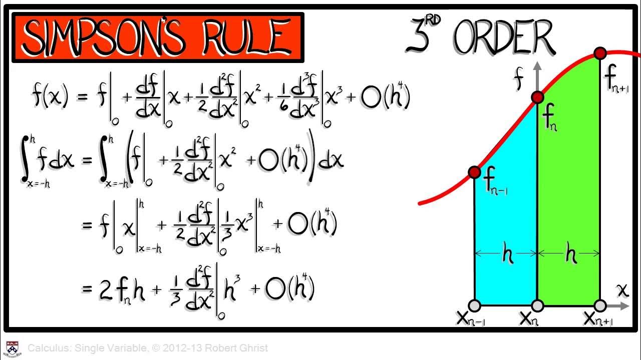
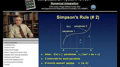
📊 Simpson's rule provides a more accurate approximation by using a pattern of coefficients 4, 2, 4, 2, ..., with the first and last terms having a coefficient of 1.
🌟 For the given example of x^2 from 0 to 8, all three methods yield approximations very close to the exact value, demonstrating their effectiveness.
🧩 The video also addresses solving word problems and finding error bounds associated with the trapezoidal and Simpson's rules.
🔍 To approximate the integration of x^3 from 1 to 9, the midpoint rule with 8 rectangles gives an approximation of 1630, close to the exact value of 1640.
📝 The script includes an example of estimating the total volume of water流出 from a tank in the first 30 minutes using the three rules, all yielding the same result of 392 gallons.
🏃‍♂️ Another example provided is estimating the distance a runner travels in the first 32 seconds using the midpoint and trapezoidal rules, with results of 255.2 meters and 243.8 meters, respectively.
🔢 The video concludes with a problem on determining the necessary value of n to ensure the midpoint rule approximation is accurate within 0.0001 for a given integral.

Q & A

What are the main numerical integration methods discussed in the video?
-The main numerical integration methods discussed in the video are the midpoint rule, trapezoidal rule, and Simpson's rule.
How is the midpoint rule used to approximate the area under a curve?
-The midpoint rule uses rectangles to approximate the area under a curve. It calculates the area of each rectangle formed by the curve and a set of horizontal lines (midpoints) and then sums these areas to get an approximation of the total area under the curve.
What is the formula for the trapezoidal rule?
-The formula for the trapezoidal rule is given by: T_n = (Δx / 2) * [f(x_0) + 2f(x_1) + 2f(x_2) + ... + 2f(x_{n-1}) + f(x_n)], where f(x_i) represents the function value at xi, and Δx is the width of the interval between successive points.
How does Simpson's rule differ from the midpoint and trapezoidal rules?
-Simpson's rule uses a combination of quadratic and linear interpolation to approximate the area under a curve. It involves a alternating pattern of coefficients (1, 4, 2, 4, ..., 1) for the function values at each interval, which helps to better capture the shape of the curve and provide a more accurate approximation.
What is the error formula for the midpoint rule?
-The error formula for the midpoint rule is given by: E <= (k * (b - a)^3) / (24 * n^2), where E is the error, k is the maximum value of the second derivative in the interval, a and b are the limits of integration, and n is the number of subintervals.
How does the error formula for the trapezoidal rule differ from that of the midpoint rule?
-The error formula for the trapezoidal rule is given by: E <= (k * (b - a)^3) / (12 * n^2). The main difference from the midpoint rule's error formula is that the denominator is 12n^2 instead of 24n^2, indicating that the trapezoidal rule requires a higher number of subintervals for the same level of accuracy.
What is the significance of the value 'n' in the context of numerical integration methods?
-The value 'n' represents the number of subintervals used in the numerical integration methods. Increasing 'n' generally improves the accuracy of the approximation, as it reduces the width of each subinterval and allows for a better fit to the curve being integrated.
How does the video demonstrate the application of the numerical integration methods?
-The video demonstrates the application of the numerical integration methods by first calculating the exact area under a curve (e.g., x^2 from 0 to 8), and then using the midpoint rule, trapezoidal rule, and Simpson's rule to approximate this area. The results from these methods are compared to the exact value to illustrate their accuracy.
What is the maximum value of the second derivative in the given example for the midpoint rule?
-The maximum value of the second derivative in the given example for the midpoint rule is 2, which occurs at the endpoint x = 1.
How does the video ensure that the numerical integration methods are accurate for the given examples?
-The video ensures accuracy by comparing the numerical integration results with the exact values obtained by integrating the given functions. It also discusses the error associated with each method and shows how to choose the number of subintervals 'n' to achieve a desired level of accuracy.
What is the exact value of the integral of x^3 from 1 to 9?
-The exact value of the integral of x^3 from 1 to 9 is 1640, which is calculated by evaluating the antiderivative, x^4/4, at the limits of integration (9 and 1) and subtracting the results.

Outlines

00:00

📚 Introduction to Numerical Integration Techniques

This paragraph introduces various numerical integration methods such as the midpoint rule, trapezoidal rule, and Simpson's rule. It also mentions the importance of these techniques in solving word problems and handling cases where the exact integration of a function is not feasible. The paragraph begins with an example of calculating the area under the curve of x^2 from 0 to 8, using the exact integration method to establish a baseline for comparison with the approximation techniques.

05:01

📐 Midpoint Rule and Trapezoidal Rule Demonstration

The paragraph demonstrates the application of the midpoint rule and trapezoidal rule to approximate the area under the curve of x^2 from 0 to 8. It explains the process of dividing the interval into sub-intervals and using rectangles to approximate the area. The midpoint rule uses the midpoints of these intervals, while the trapezoidal rule incorporates both the first and last points of each sub-interval, providing a more accurate approximation. The results from both methods are compared to the exact answer, showing their effectiveness.

10:03

📊 Simpson's Rule and its Application

This paragraph introduces Simpson's rule, a more advanced numerical integration technique that provides even greater accuracy. It explains the formula for Simpson's rule and its application to the same function used in the previous paragraphs. The example calculation shows how to apply the rule to approximate the integral of x^2 from 0 to 8, and the result is compared to the exact answer, demonstrating the high precision of Simpson's rule.

15:13

🔢 Approximating Integrals with Different Functions

The paragraph presents a new example of approximating the integral of x^3 from 1 to 9 using the midpoint rule, trapezoidal rule, and Simpson's rule. It explains the process of finding the exact value of the integral and then using the numerical methods to approximate it. The results from each method are compared, showing that all three techniques yield close approximations to the exact value, with Simpson's rule providing the most accurate result.

20:15

🏗️ Applying Numerical Integration to Real-World Problems

This paragraph applies the numerical integration techniques to a practical problem of estimating the volume of water flowing out of a tank based on a given data table. It demonstrates how to use the trapezoidal rule, Simpson's rule, and the midpoint rule to approximate the integral, which in this context represents the volume of water. The example shows that all three methods can be effectively used to solve real-world problems, providing accurate estimations of the total volume of water after a given time period.

25:18

🏃‍♂️ Estimating Distance with Numerical Integration

The paragraph discusses the use of numerical integration methods to estimate the distance traveled by a runner based on a data table of their speed over time. It outlines the process of applying the midpoint rule and trapezoidal rule to the given data, calculating the estimated distance covered by the runner in the first 32 seconds. The example illustrates how these integration techniques can be used to analyze and interpret data in a practical scenario.

30:19

🔍 Ensuring Accuracy in Numerical Integration

This paragraph delves into the error analysis associated with the midpoint rule, providing a formula to estimate the error and ensure the accuracy of the approximation. It explains how to determine the value of n needed to achieve a certain level of accuracy, using a specific example of approximating an integral with a given error tolerance. The paragraph emphasizes the importance of understanding the error bounds when using numerical integration methods.

35:23

📈 Using Trapezoidal Rule with a Specific n Value

The paragraph focuses on applying the trapezoidal rule with a specific value of n to approximate an integral. It explains the process of calculating the integral of x^3 from 1 to 2 using n equals four, detailing the steps of finding the function values at the points of interest and the error associated with this approximation. The example demonstrates how to work through the trapezoidal rule method and interpret the results, including the error bounds.

Mindmap

Keywords

💡Integration

Integration in the context of the video refers to the mathematical process of finding the area under a curve, which is represented by the integral of a function. It is a fundamental concept in calculus and is used to solve a variety of problems, including those related to rates of change and accumulation. The video discusses approximating integration when an exact solution is not possible using methods like the midpoint rule, trapezoidal rule, and Simpson's rule.

💡Midpoint Rule

The midpoint rule is a numerical method used to approximate the definite integral of a function. It involves dividing the interval into equal subintervals and using the midpoint of each subinterval to calculate the area under the curve. The video explains how to apply the midpoint rule by choosing four rectangles to approximate the area under the curve of x^2 from 0 to 8, resulting in a sum of the function values at the midpoints multiplied by the width of the rectangles.

💡Trapezoidal Rule

The trapezoidal rule is another numerical method for approximating the definite integral of a function. It works by dividing the area under the curve into a series of trapezoids and calculating the area of each trapezoid to estimate the total area. The rule is based on the idea that the sum of the areas of these trapezoids closely approximates the area under the curve. The video shows how to use the trapezoidal rule to estimate the integral of x^2 from 0 to 8 by including five points and weighing the function values at the ends and in the middle differently.

💡Simpson's Rule

Simpson's rule is a more advanced numerical method for approximating the definite integral of a function. It provides a better approximation than the midpoint and trapezoidal rules by using a parabolic fit through three points in each subinterval. The rule is based on the assumption that the function can be approximated by a parabola over small intervals, which leads to a more accurate estimation of the area under the curve. The video demonstrates Simpson's rule by evaluating the function at five points and applying the specific coefficients of the rule (1, 4, 2, 4, 1) to these values.

💡Error Bound

The error bound refers to the maximum amount by which a numerical approximation can differ from the actual value. In the context of the video, it is used to quantify the accuracy of the approximations made using the midpoint rule, trapezoidal rule, and Simpson's rule. The video discusses how to calculate the error bound for these methods, which is important for determining the level of precision in the numerical integration.

💡Anti-Derivative

An anti-derivative, also known as an integral function, is a function whose derivative is equal to the given function. In the context of the video, finding the anti-derivative of a function is essential for calculating the exact area under the curve, which represents the integral. The anti-derivative is used to evaluate the integral by substituting the bounds of the interval and finding the difference in the function values at these bounds.

💡Approximation

Approximation in the video refers to the process of estimating a value or quantity that is not exactly known or cannot be precisely calculated. The video focuses on approximating the integral of a function when an exact solution is not feasible. The approximation is achieved through numerical methods like the midpoint rule, trapezoidal rule, and Simpson's rule, which provide close estimates of the actual integral value.

💡Delta X (Δx)

Delta X (Δx) represents the width of each subinterval in the numerical methods used for approximating integration. It is the difference between the endpoints of the interval divided by the number of subintervals (n). In the context of the video, Δx is a crucial parameter that affects the accuracy of the approximation, with smaller values leading to more precise estimates.

💡Rectangles

In the context of numerical integration methods discussed in the video, rectangles are used as a geometric shape to approximate the area under a curve. The methods like the midpoint rule and trapezoidal rule involve dividing the area under the curve into rectangles and calculating the sum of the areas of these rectangles to estimate the total area. The height of each rectangle is determined by the function value at a specific point, and the width is determined by Δx.

💡Data Table

A data table in the context of the video refers to a set of values that correspond to the function's output for a range of input values. It is a way to represent the function's behavior in a tabular form, which can be used for numerical integration methods. The video discusses how to use data tables in conjunction with the trapezoidal and midpoint rules to estimate integrals when direct integration is not possible or practical.

💡Volume Flow Rate

Volume flow rate refers to the rate at which a volume of fluid, such as water, flows through a given cross-sectional area per unit of time. In the video, it is used in the context of a practical problem where the flow rate of water leaving a tank is given, and the task is to estimate the total volume of water that has flowed out over a certain period using numerical integration methods like the trapezoidal and midpoint rules.

Highlights

Introduction to approximating integration using the midpoint rule, trapezoidal rule, and Simpson's rule.

Explanation of how to solve word problems involving integration approximation.

Method to find the error bound of the trapezoidal rule.

Process to solve problems with the error bound of Simpson's rule.

Exact calculation of the area under the curve for the function x squared from 0 to 8.

Approximation of the area under the curve using the midpoint rule.

Estimation of the area using the trapezoidal rule and its closeness to the actual value.

Application of Simpson's rule and its remarkable accuracy.

Integration of x cubed from 1 to 9 using the exact method.

Comparison of the midpoint rule, trapezoidal rule, and Simpson's rule in approximating the integral of x cubed.

Demonstration of estimating the total volume of water flowed out of a tank using the trapezoidal and Simpson's rules.

Use of the midpoint rule to estimate the distance traveled by a runner.

Estimation of the distance in meters using the trapezoidal rule for a runner's speed data.

Determination of the necessary value of n for the midpoint rule to guarantee accuracy within .0001.

Application of the trapezoidal rule with n equals four and calculation of the error range.

Verification of the trapezoidal rule's approximation against the actual integral value.

Transcripts

Browse More Related Video

Numerical Integration With Trapezoidal and Simpson's Rule

Calculus Chapter 5 Lecture 49 Numerical Integration II

Lec 25 | MIT 18.01 Single Variable Calculus, Fall 2007

5.7 Numerical Integration (Quadrature)

Lec 24 | MIT 18.01 Single Variable Calculus, Fall 2007

Calculus AB Homework 6.2 Riemann and Trapezoidal Sums

Related Tags

Numerical Integration Midpoint Rule Trapezoidal Rule Simpson's Rule Integral Approximation Word Problems Error Bounds Calculus Techniques Mathematical Analysis Educational Content