Linear Regression and Correlation - Example
TLDRThis video script delves into the concept of linear regression and correlation using a set of six paired data points. It guides viewers through the process of constructing a table to calculate the sum of X, Y, X squared, Y squared, and XY values. The script explains how to derive the line of best fit using the least squares method and determine the correlation coefficient to measure the strength of the linear relationship. The video also distinguishes between interpolation and extrapolation, cautioning against the latter due to potential inaccuracies outside the observed data range.
Takeaways
- 📈 The video discusses an example of linear regression and correlation using six pairs of data for two variables, x and y.
- 🔍 The purpose is to determine if there is a linear relationship between the two variables and the strength of that relationship.
- 📊 A table is constructed to calculate the sums of x, y, x squared, y squared, and the product of x and y (x*y).
- 🧮 The line of least squares (regression line) is calculated using the formula for the slope (a hat) and y-intercept (b hat) based on the column totals.
- 📚 The coefficient of correlation is used to measure the strength of the linear relationship, with values close to 1 indicating a strong correlation.
- 🔢 The standard deviation for the sample of x and y values is calculated to help determine the coefficient of correlation.
- 📉 The slope of the line of least squares is found to be approximately 0.93244, and the y-intercept is approximately 0.3808.
- 🔎 The coefficient of correlation (R) is calculated to be approximately 0.94777, indicating a very strong linear relationship.
- 🔍 Interpolation is used to predict y values for x values within the observed range, while extrapolation is cautioned against as it may not hold the same linear relationship.
- 📚 The video concludes with examples of interpolation, demonstrating how to predict y values for x values within the observed range and vice versa.
Q & A
What is the main topic of the video?
-The main topic of the video is to demonstrate how to find the line of best fit for a set of data points using linear regression and to determine the correlation between two variables using the coefficient of correlation.
What are the two variables in the given data pairs?
-The two variables in the given data pairs are x and y, which could represent any two related quantities, such as the change in stock prices over time.
How many pairs of data are provided in the script?
-There are six pairs of data provided in the script.
What is the purpose of creating a table with sums of x, y, x squared, y squared, and x times y?
-The table with these sums is used to compute the line of least squares and the coefficient of correlation, which are essential for understanding the linear relationship between the variables.
What is the formula for calculating the slope (a hat) of the line of least squares?
-The formula for calculating the slope (a hat) is given by (Σ(x * y) - n * (Σx * Σy)) / (Σ(x^2) - n * (Σx)^2), where n is the number of data pairs.
What is the formula for calculating the y-intercept (b hat) of the line of least squares?
-The formula for calculating the y-intercept (b hat) is given by (Σx * Σy - Σ(x * y) * Σx) / (Σ(x^2) - n * (Σx)^2), where n is the number of data pairs.
What does the coefficient of correlation measure?
-The coefficient of correlation measures the strength and direction of the linear relationship between two variables. It ranges from -1 to 1, with values close to 1 indicating a strong positive correlation.
What is the difference between interpolation and extrapolation in the context of the video?
-Interpolation refers to predicting a value within the range of observed data points, while extrapolation refers to predicting a value outside the range of observed data points. The video emphasizes caution when using extrapolation due to the potential for the linear relationship to break down outside the observed range.
What is the approximate slope of the line of least squares calculated in the video?
-The approximate slope of the line of least squares calculated in the video is 0.9304.
What is the approximate y-intercept of the line of least squares calculated in the video?
-The approximate y-intercept of the line of least squares calculated in the video is 0.3808.
How is the coefficient of correlation calculated in the video?
-The coefficient of correlation is calculated using the formula R = Σ(x * y) - (Σx * Σy) / (n * s_x * s_y), where n is the number of data pairs, s_x and s_y are the standard deviations of x and y respectively.
What is the significance of the standard deviation of x and y in calculating the coefficient of correlation?
-The standard deviations of x and y are used to normalize the data, allowing the coefficient of correlation to be calculated in a way that is independent of the units of measurement of x and y.
Outlines
📊 Introduction to Linear Regression and Correlation
The video begins with an introduction to the concepts of linear regression and correlation using a set of six paired data points for two variables, x and y. The variables could represent any two related phenomena, such as the performance of two stocks at different times. The goal is to determine if there is a linear relationship between the variables and to quantify the strength of this relationship using the line of least squares and the coefficient of correlation. The process involves creating a table to summarize the data, including sums of x and y values, their squares, and cross-products, which will be used to calculate the regression line and the correlation coefficient.
🔍 Calculating the Line of Least Squares
This paragraph explains the method to calculate the slope (a hat) and y-intercept (b hat) of the line of least squares using the previously computed column totals and the number of data pairs (n). The formula for the slope is given by the difference between the product of the sums of x and y, and the product of n and the sum of the cross terms, divided by the difference between the square of the sum of x and n times the sum of the squares of x. The y-intercept is calculated similarly, with a different numerator but the same denominator. The calculated values for the slope and y-intercept are then used to form the equation of the line of least squares, which is essential for making predictions about the relationship between the variables.
📉 Understanding the Coefficient of Correlation
The coefficient of correlation, denoted as 'R', measures the strength and direction of the linear relationship between the two variables. To compute 'R', the standard deviations of the sample x and y values are first calculated using a shortcut formula based on the summations of the data. The coefficient of correlation is then found either by using the previously calculated slope (a hat) and the standard deviations or by using a direct formula that involves the sums of x and y, their means, and the standard deviations. A high absolute value of 'R' indicates a strong correlation, suggesting that the line of least squares can be used to make accurate predictions.
🔮 Making Predictions with Linear Regression
With the line of least squares and a strong coefficient of correlation, the video discusses how to use the regression line for making predictions, specifically through interpolation and extrapolation. Interpolation involves predicting a y value for an x within the observed range, while extrapolation extends predictions beyond the observed range. The video emphasizes the importance of staying within the observed range for reliable predictions and cautions against extrapolation due to the potential breakdown of the linear relationship outside the observed data range.
📌 Examples of Interpolation and Extrapolation
The final paragraph provides examples to illustrate the concepts of interpolation and extrapolation. Interpolation is demonstrated by predicting a y value when x is within the observed range, using the line of least squares equation. Extrapolation is discussed as predicting a y value for an x outside the observed range, which is not recommended due to the uncertainty of the linear relationship holding true. Additionally, the video shows how to perform 'backwards' interpolation, where an observed y value is used to predict an x value, again within the observed range of y values.
Mindmap
Keywords
💡Linear Regression
💡Correlation
💡Coefficient of Correlation
💡Least Squares
💡Slope
💡Y-Intercept
💡Standard Deviation
💡Interpolation
💡Extrapolation
💡Stock Variables
Highlights
Introduction of a linear regression and correlation example with six pairs of data.
Explanation of potential real-world applications, such as stock price trends, for the variables x and y.
The method to determine if a linear relationship exists between two variables using the line of least squares.
The importance of the coefficient of correlation in measuring the strength of a linear relationship.
Step-by-step guide to constructing a table for sum of X, Y, X squared, Y squared, and X*Y values.
Calculation of the slope (a hat) of the least squares line using the formula and given data totals.
Determination of the y-intercept (B hat) using the calculated totals and the same denominator as the slope.
Derivation of the linear regression equation using the calculated slope and y-intercept.
Discussion on the accuracy of predictions made using the line of least squares based on the correlation strength.
Introduction to the concept of standard deviation for a sample and its calculation.
Explanation of how to compute the coefficient of correlation using the slope of the least squares line.
Alternative method to find the coefficient of correlation without relying on the slope.
Interpretation of a strong correlation coefficient indicating accurate predictions from the regression line.
Illustration of interpolation using the regression line to predict within the observed range of x values.
Caution against extrapolation when predicting outside the observed range of x values due to potential inaccuracies.
Example of backward interpolation to predict x values from an observed y value within the range.
Final thoughts on the reliability of using the regression line for predictions within the observed data range.
Transcripts
Browse More Related Video
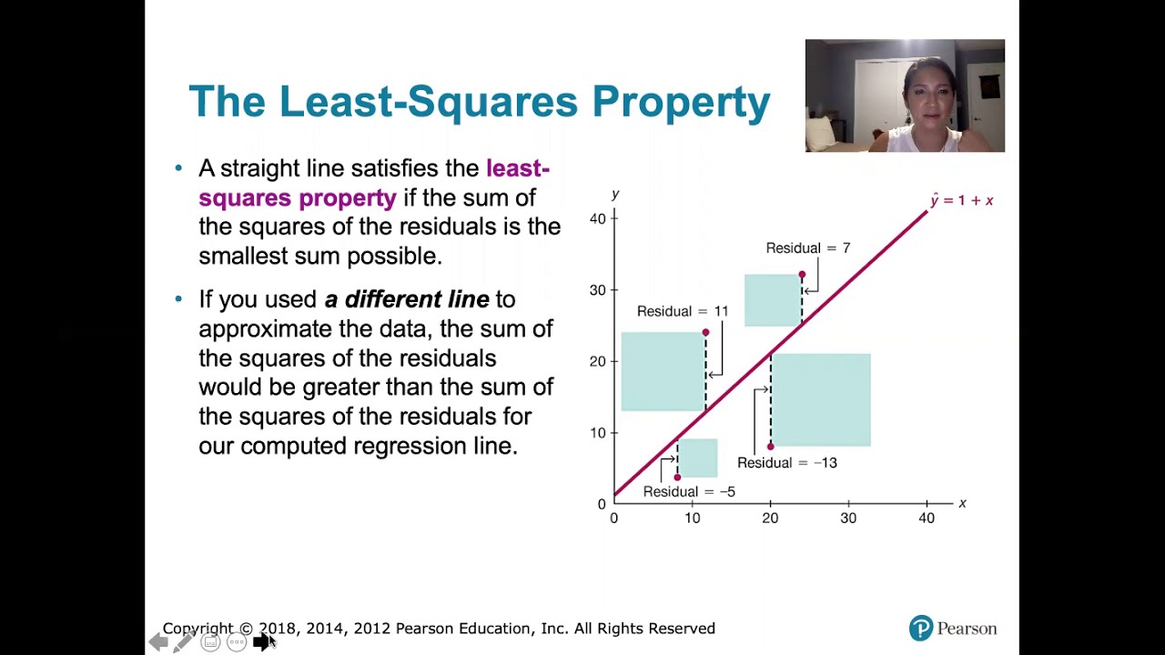
10.2.5 Regression - Residuals and the Least-Squares Property

Elementary Stats Lesson #6

Elementary Stats Lesson #5

Linear Regression and Correlation - Introduction
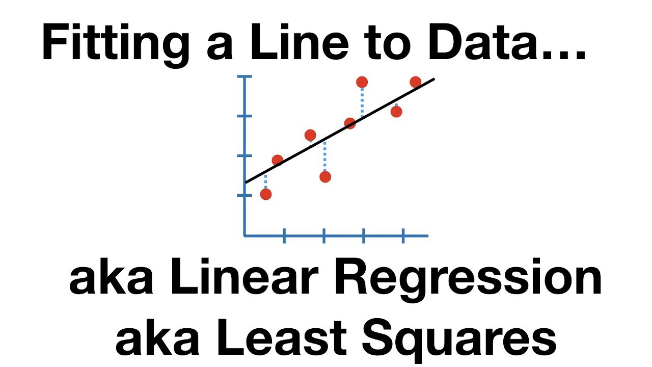
The Main Ideas of Fitting a Line to Data (The Main Ideas of Least Squares and Linear Regression.)
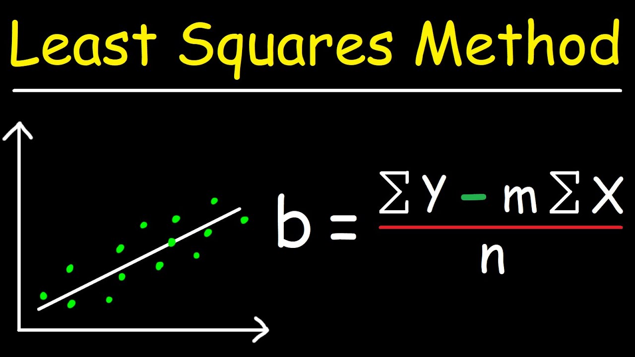
Linear Regression Using Least Squares Method - Line of Best Fit Equation
5.0 / 5 (0 votes)
Thanks for rating: