Business Calculus -- Math 1329 -- Section 4.2 -- Logarithmic Functions
TLDRThis video script delves into the world of logarithmic functions, starting with the basics of what a logarithm is and how it's notated. It explains the relationship between logarithms and exponential functions, using examples to illustrate how to simplify logarithmic expressions. The script moves on to explore the properties of logarithms, including the rules for combining them and the base-changing formula. It also covers how to simplify and expand logarithmic expressions, emphasizing the importance of understanding logarithmic properties. The video then transitions into graphing logarithmic functions, discussing their general properties and how the graph changes with different bases. Practical applications are introduced with examples of solving logarithmic equations and modeling population growth using exponential functions. The script concludes with a step-by-step guide to finding an exponential model to predict future population sizes and determine the time it takes for a population to double. Throughout, the video emphasizes the mathematical concepts and problem-solving strategies essential for understanding logarithms and their applications.
Takeaways
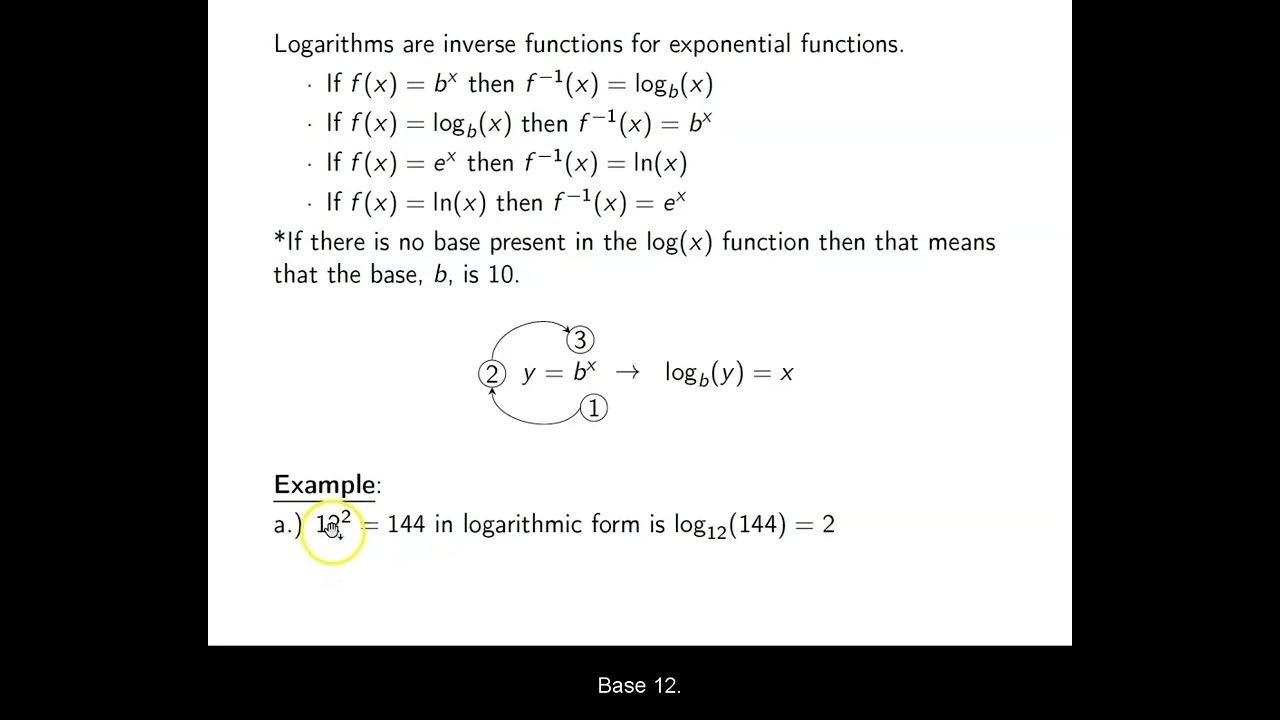
- 📖 The notation for a logarithm is y = log_B(x), which can be rewritten as B^y = x, showing the relationship between logarithms and exponential functions.
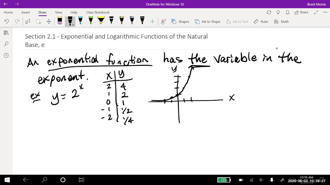
- 🔍 A logarithm essentially represents the exponent needed to raise the base B to in order to get the value x.
- 🌰 Example 1: log_2(8) = 3 because 2 × 2 × 2 = 8.
- 🌰 Example 2: log_5(5^9) = 9 because 5^9 is 5 raised to the 9th power.
- 🌰 Example 3: log_7(√[3]{7}) = 1/3 because the cube root of 7 can be written as 7^{1/3}.
- 📢 The common logarithm (base 10) is often used in scientific notation and is denoted without a base, as in log(10000) = 4.
- ℓ The natural logarithm, denoted as ln(e), has a base e and is equal to 1 because e^1 = e.
- ➕➖ Logarithm properties include: log_B(x) + log_B(y) = log_B(xy), log_B(x) - log_B(y) = log_B(x/y), (log_B(x))^r = r · log_B(x), and log_B(B^r) = r.
- 🔄 The base changing formula allows you to evaluate logarithms with different bases, such as log_B(x) = log_C(x)/log_C(B).
- 📈 When graphing y = log_B(x), for B > 1, the graph has a vertical asymptote at x = 0, passes through (1,0) and (B,1), and increases from negative infinity to positive infinity as x increases.
- 📉 For 0 < B < 1, the graph is a mirror image over the x-axis, with a vertical asymptote at x = 0, and the limit as x approaches zero from the right is positive infinity, while as x approaches infinity, the limit is negative infinity.
- 🔧 To solve logarithmic equations, revert to exponential form, isolate the variable, and solve for the variable, as demonstrated in the examples provided.
Q & A
What is the notation for a logarithm?
-The notation for a logarithm is y = log base B of X, which can be switched around to B raised to the Y power is equal to X.
How are logarithmic functions and exponential functions related?
-Logarithmic functions and exponential functions are intimately related. The log base B of X is equal to Y, and Y becomes the exponent when you look at the exponential version of the function (B raised to the Y power equals X).
What is the value of log base two of eight?
-The value of log base two of eight is three, because two to the third power (2 x 2 x 2) equals eight.
What is the value of the common log of 10,000?
-The common log (base 10) of 10,000 is equal to 4, because 10 to the fourth power (10 x 10 x 10 x 10) equals 10,000.
What is the natural log of E?
-The natural log of E (base e) is 1, because e to the first power equals e.
What are the logarithm properties for B > 0 and B not equal to 1, with x and y positive real numbers?
-The properties include: log base B of X plus log base B of Y equals log base B of X times Y, log base B of X minus log base B of Y equals log base B of X over Y, log base B of X to the R power equals R times log base B of X, and log base B of B raised to the R power equals R.
What is the base changing formula for logarithms?
-The base changing formula is log base B of X equals log base C of X divided by log base C of B. It is used to evaluate logarithms when the base is not directly available on a calculator.
How can you simplify the expression five log base two of X minus 3 log base two of Y plus one half log base 2 of Z?
-You can simplify the expression to a single logarithm: log base 2 of (X to the fifth power times the square root of Z) divided by (Y cubed).
What is the domain and range of the logarithmic function y = log base B of X when B > 1?
-The domain is 0 to infinity (since you cannot take the log of 0 or a negative number), and the range is all real numbers as the function continues to rise without leveling off.
What is the general shape of the graph of y = log base B of X when B > 1?
-The graph has a vertical asymptote at X equals 0, starts at negative infinity, rises, and then curves around, passing through the points (1, 0) and (B, 1).
How do you solve for X in the equation log base 3 of (2X - 1) equals 2?
-Revert to exponential form to get 3 squared equals 2X - 1. Solving gives 2X = 10, hence X equals 5.
How do you find the exponential model to predict the population, given the population in the years 2000 and 2010?
-Use the given population figures to create two points (T, P), where T is the number of years since 2000. Then apply the model P = P naught e raised to the RT power, and solve for the growth rate R using the points provided.
Outlines
📚 Introduction to Logarithms
This paragraph introduces the concept of logarithms, explaining the notation and relationship with exponential functions. It demonstrates how to simplify logarithmic expressions through examples, such as finding the log base two of eight or the log base five of five to the ninth power. It also covers the concept of the common logarithm (base 10) and the natural logarithm (base e), and presents basic properties and rules of logarithms, including the product rule, quotient rule, power rule, and the base change formula.
🔢 Logarithm Properties and Simplification
The second paragraph delves into logarithmic properties, discussing how to add, subtract, and raise to a power within logarithmic expressions. It provides a method for simplifying multiple logarithms into a single logarithm by converting coefficients into powers and applying the rules of logarithms. An example is given to illustrate the process of combining logarithms with different coefficients into one expression.
📈 Graphing Logarithmic Functions
This paragraph focuses on the graphical representation of logarithmic functions. It explains the general shape of the graph for a logarithm with a base greater than 1, including the vertical asymptote at x=0, the domain and range, and key points the graph passes through. It also discusses the behavior of the graph as x approaches zero and infinity and contrasts this with the graph for a base between 0 and 1.
🧮 Solving Logarithmic Equations
The fourth paragraph presents strategies for solving logarithmic equations, starting with reverting to exponential form. It provides examples of solving for x in different logarithmic equations, including using properties of logarithms to isolate the variable and using natural logs to bring down exponents to the base level. The paragraph also touches on the application of these methods in exponential models for predicting population growth.
📊 Exponential Growth Model and Predictions
This paragraph discusses the application of exponential growth models to predict population growth. It outlines the steps to derive the growth rate (R) from given population data points, using the model P = P0 * e^(RT), where P0 is the initial population, R is the growth rate, and T is time. The paragraph demonstrates how to use the model to predict future population and calculate the time required for the population to double, emphasizing the use of exact values and the sensitivity of the growth rate to the number of decimal places used.
🔁 Population Growth and Doubling Time
The final paragraph wraps up the discussion on population growth by illustrating how to use the derived exponential model to predict the population for a future year (2020) and to calculate the doubling time of the population. It emphasizes that the doubling time is consistent and depends only on the number of years, regardless of the starting population size. The paragraph concludes with a reminder of the importance of using accurate calculations for reliable predictions.
Mindmap
Keywords
💡Logarithm
💡Exponential Function
💡Base
💡Common Log
💡Natural Log
💡Logarithmic Properties
💡Graph of Logarithmic Functions
💡Exponential Growth Model
💡Vertical Asymptote
💡Domain and Range
💡Solving Logarithmic Equations
💡Population Growth
Highlights
Logarithms are the inverse operation to exponentiation, with the notation y = log base B of X, which can be rewritten as B^Y = X.
Logarithms and exponential functions are intimately related, where the exponent needed to achieve a value is represented by the logarithm.
Example 1 demonstrates simplifying log base two of eight by determining the power to which two must be raised to get eight, resulting in log base two of eight equals three.
Example 2 illustrates that log base five of five to the ninth is simply 9, as no other power of five will result in five to the ninth.
Example 3 involves rewriting the cube root of seven as a fractional exponent to find log base seven of the cube root of seven, which equals 1/3.
The common log, with base 10, is used for scientific notation and is represented without specifying the base, as seen when finding the log of 10,000.
The natural log, denoted as ln, has the base e and is used to find the power to which e must be raised to get e, which is 1.
Logarithmic properties include the ability to add or subtract logs by multiplying or dividing their arguments, and to bring powers outside of the log.
The base changing formula allows for the evaluation of logs with different bases, such as log base 12, using natural log or common log.
Simplifying multiple logarithms involves converting coefficients into powers and combining arguments through multiplication or division based on the signs.
Expanding logarithms involves using the reverse of the logarithmic properties to distribute a single log across multiple terms.
The graph of a logarithmic function with base greater than 1 has a vertical asymptote at x=0, a domain of (0, ∞), and a range of all real numbers.
For a base between 0 and 1, the graph of the logarithmic function is a mirror image over the x-axis compared to when the base is greater than 1.
Solving logarithmic equations often involves reverting to exponential form, as shown in example 5 where log base 3 of 2x minus 1 equals 2.
In example 6, solving for x in an exponential equation involves using natural logs to isolate the variable in the exponent.
An exponential model for population growth can be found using the formula P = P0 * e^(RT), where P0 is the initial population, R is the growth rate, and T is time.
Predicting future population or determining the time for population doubling involves solving the exponential model for the desired year or using the natural log to find the time variable.
The rate of population increase in an exponential model is constant and does not depend on the starting population, making the time to double a consistent figure.
Transcripts
Browse More Related Video
Ch. 4.3 Logarithmic Functions
Math 11 - Section 2.1
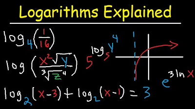
Logarithms Explained Rules & Properties, Condense, Expand, Graphing & Solving Equations Introduction
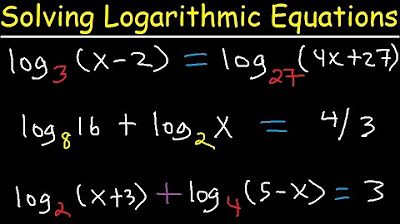
Solving Logarithmic Equations With Different Bases - Algebra 2 & Precalculus

2.3 - Derivatives of Logarithmic Functions
Calculus 2 Lecture 6.3: Derivatives and Integrals of Exponential Functions
5.0 / 5 (0 votes)
Thanks for rating: