How to Calculate Residual Sum of Squares
TLDRThis video script introduces the concept of residual sum of squares, a key parameter for validating the linearity of methods. It explains the calculation of residuals as the difference between observed and predicted values in a linearity experiment, using a hypothetical HPLC method as an example. The script demonstrates how to use Excel functions to calculate the slope and y-intercept of a linear line, and then how to apply these to find the residuals for different concentration levels. Finally, it shows the process of squaring the residuals and summing them up to obtain the residual sum of squares, emphasizing its importance in assessing method linearity.
Takeaways
- 📈 Residual Sum of Squares (RSS) is a crucial parameter for establishing linearity in method validation.
- 🔍 Linearity study involves understanding the correlation coefficient, y-intercept, slope, and RSS.
- 📊 In an HPLC linearity experiment, concentration is plotted on the x-axis and peak area on the y-axis.
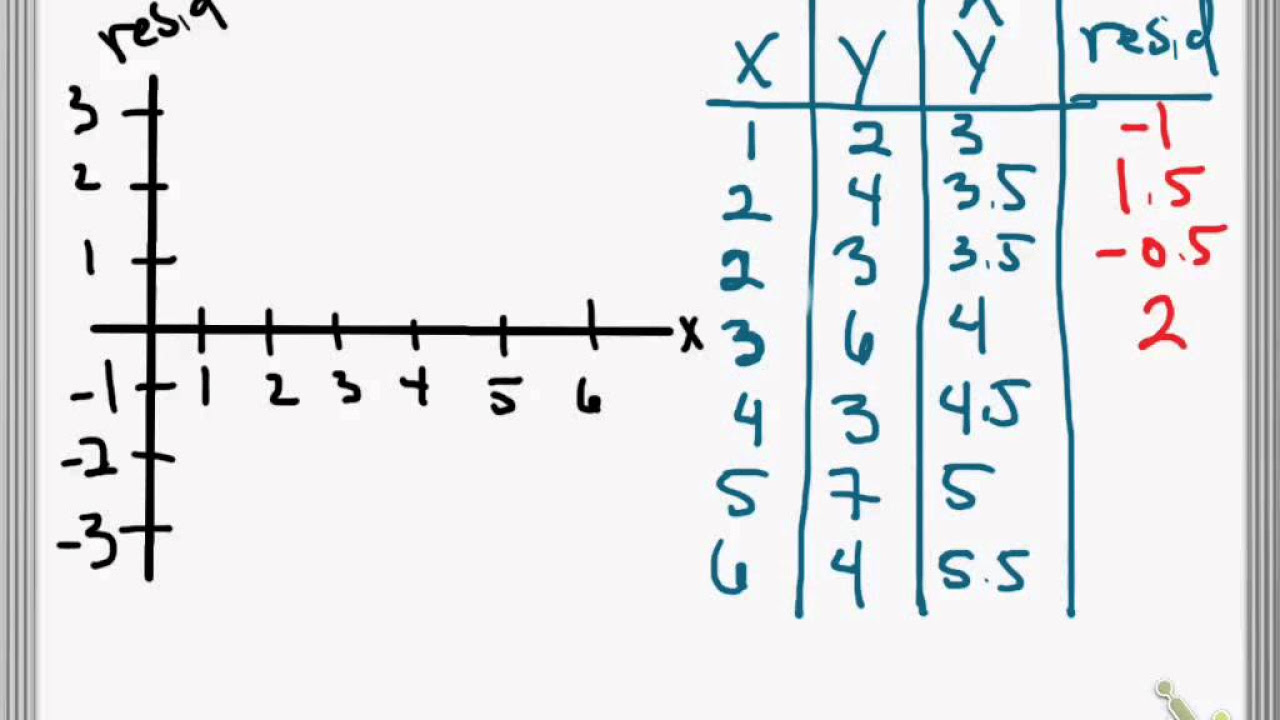
- 📌 Residual is the deviation of the observed response from the predicted response.
- ➕ Positive residuals occur when the deviation is above the regression line, and negative residuals are when deviations are below the line.
- 🔢 The formula for calculating residuals is: Residual = Observed Value - (m*x + c), where m is the slope, x is the concentration, and c is the y-intercept.
- 📱 Predicted values are calculated using the linear equation y = mx + c.
- 🔧 Excel can be used to calculate the slope and y-intercept, but not directly for RSS.
- 💻 To calculate RSS in Excel, first find the residuals for each concentration level, then square each residual, and finally sum all squared residuals.
- 🎯 The sum of all residuals should be close to zero, as the regression line is designed to minimize the deviation between observed and predicted values.
- 👋 The video provides a clear explanation of how to calculate RSS as part of a linearity study.
Q & A
What is the residual sum of squares?
-The residual sum of squares is a parameter used to establish the linearity as part of method validation. It measures the difference between the observed values and the predicted values in a linearity experiment.
What are the three parameters involved in the linearity study?
-The three parameters involved in the linearity study are the correlation coefficient, the y-intercept, and the slope.
How can the correlation coefficient, y-intercept, and slope be established?
-These parameters can be established using Excel set functions. The correlation coefficient and slope can be calculated using the relevant Excel formulas, while the y-intercept can be determined from the linear equation.
What is the formula for calculating residuals?
-The formula for calculating residuals is the observed value minus the predicted value (residual = observed value - (mx + c)), where m is the slope, x is the independent variable (e.g., concentration), and c is the y-intercept.
How do you calculate the predicted value in the context of the linearity study?
-The predicted value is calculated using the equation of the linear line, y = mx + c, where y is the predicted value, m is the slope, x is the independent variable (e.g., concentration), and c is the y-intercept.
What does a positive residual indicate?
-A positive residual indicates that the observed value is above the regression line by a certain number of units, representing a deviation from the predicted response.
What does a negative residual indicate?
-A negative residual indicates that the observed value is below the regression line by a certain number of units, also representing a deviation from the predicted response.
How is the residual sum of squares calculated?
-The residual sum of squares is calculated by squaring each residual (difference between observed and predicted values) and then summing up all the squared residuals.
What is the property of the sum of residuals?
-The sum of residuals will always be close to zero, as the regression line is drawn in such a way that the total deviation (distance) from each point to the line is minimized.
Why is the residual sum of squares an important parameter in the linearity study?
-The residual sum of squares is an important parameter because it provides a measure of how well the observed data fits the predicted linear model. A lower residual sum indicates a better fit and more reliable linear relationship.
How can you practically calculate the residuals and the residual sum of squares using Excel?
-You can calculate the residuals and the residual sum of squares using Excel by first determining the slope and y-intercept, then applying the residual formula for each observed value. The squared residuals are then calculated, and their sum gives you the residual sum of squares.
Outlines
📈 Introduction to Residual Sum of Squares
This paragraph introduces the concept of residual sum of squares, which is a crucial parameter for validating the linearity of methods. It explains that this parameter, along with the correlation coefficient, y-intercept, and slope, is vital for understanding the linearity study. The explanation begins with a discussion on how to calculate the residual sum of squares and proceeds to define the term 'residual' using an example of a linearity experiment in an HPLC method. The paragraph highlights the importance of understanding the observed and predicted values and how deviations from the regression line are categorized as positive or negative residuals.
🧮 Calculation of Residuals and Predicted Values
This paragraph delves into the specifics of calculating residuals and predicted values. It provides a clear explanation of how to determine the slope and y-intercept using Excel functions, which are essential for calculating the predicted values. The paragraph uses a hypothetical example with different concentration levels and corresponding peak areas to illustrate the calculation of residuals. It emphasizes the importance of understanding the relationship between the independent variable (concentration) and the dependent variable (peak area) and how this relationship is used to calculate the residuals for each data point.
📊 Residual Sum of Squares and its Implications
The final paragraph discusses the calculation of the residual sum of squares, which is the summation of the squares of the residuals. It explains the process of squaring each residual and then summing them up to obtain the residual sum of squares. The paragraph also touches on the property of residuals that their sum equals zero, highlighting the efficiency of the regression line in minimizing the overall deviation from the observed points. The explanation concludes with a summary of the key points discussed in the video, reinforcing the importance of understanding the calculation and significance of the residual sum of squares in the context of linearity studies.
Mindmap
Keywords
💡Residual Sum of Squares
💡Linearity
💡Correlation Coefficient
💡Y-Intercept
💡Slope
💡HPLC Method
💡Concentration Levels
💡Peak Area
💡Regression Line
💡Excel Functions
Highlights
The video discusses the calculation of the residual sum of squares, a key parameter in establishing methods linearity as part of method validation.
Residual sum of squares is a measure used to understand the deviation of observed values from the predicted values in a linearity experiment.
In a linearity study, concentration is plotted against the x-axis and peak area against the y-axis, with deviations from the predicted response being noted.
The observed deviation from the predicted response is termed as the residual, which can be either positive or negative depending on whether it is above or below the regression line.
The formula for calculating residuals is the observed value minus the predicted value (y = mx + c), where m is the slope, x is the independent factor (concentration), and c is the y-intercept.
Excel can be used to calculate the correlation coefficient, y-intercept, and slope, but not the residual sum of squares, which requires a specific formula.
The video provides a step-by-step guide on how to calculate residuals and the residual sum of squares using an example of an HPLC method.
The example given involves five different concentration levels (A, B, C, D, E) and their corresponding peak areas, with residuals calculated for each level.
The video demonstrates how to use Excel functions to calculate the slope and y-intercept, which are essential for determining the predicted value from the observed concentration and peak area.
The residual sum of squares is calculated by summing the squares of the residuals, which is a measure of the total deviation of the observed points from the regression line.
The video emphasizes that the summation of residuals should always be close to zero, as the regression line is drawn to minimize the distance between each point and the line.
The calculation of the residual sum of squares is crucial for the estimation of linearity parameters and the validation of analytical methods.
The video concludes by reinforcing the importance of understanding the calculation of the residual sum of squares for method linearity estimation.
The presenter expresses a commitment to providing useful and informative content, promising more videos on similar topics in the future.
Transcripts
Browse More Related Video

How to Calculate the Residual

10.2.5 Regression - Residuals and the Least-Squares Property
Residuals and Residual Plots
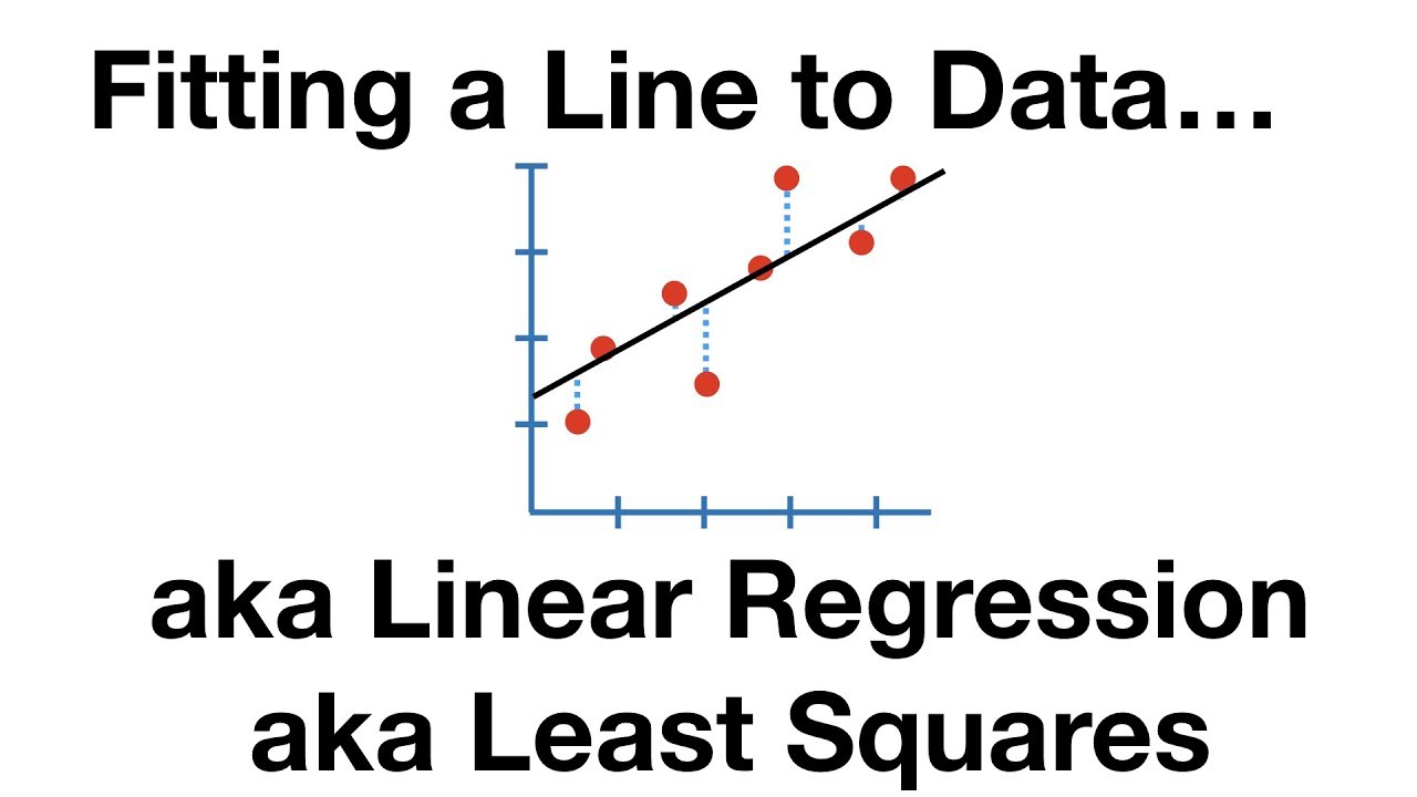
The Main Ideas of Fitting a Line to Data (The Main Ideas of Least Squares and Linear Regression.)

Residual plots | Exploring bivariate numerical data | AP Statistics | Khan Academy

Calculating Residuals and MSE for Regression by hand
5.0 / 5 (0 votes)
Thanks for rating: