Standard Error (of the sample mean) | Sampling | Confidence Intervals | Proportions
TLDRIn this final installment of the descriptive statistics series, the focus is on the standard error of the sample mean, a concept that bridges basic descriptive measures with more advanced statistics. The video explains the standard error as a measure of uncertainty in the sample mean, which decreases as the sample size increases. It is calculated using the formula \\ ( SE = \frac{s}{\sqrt{n}} \\ ), where \\ ( s \\ ) is the standard deviation and \\ ( n \\ ) is the sample size. The script delves into confidence intervals, illustrating how they provide a range within which the population mean is expected to fall with a certain level of confidence. The video also explores the standard error of the sample proportion and its application in creating confidence intervals for categorical data. A challenge question is posed regarding the number of additional measurements needed to achieve a desired standard error, encouraging viewer engagement and discussion. The series concludes with an invitation to further explore statistics through the presenter's next video on sampling.
Takeaways
- 📊 **Standard Error Definition**: The standard error of the sample mean (SE) is a measure of the variability of the sample mean, calculated as the standard deviation (s) divided by the square root of the sample size (n).
- 🔍 **Descriptive vs. Inferential Statistics**: While standard error is not typically a descriptive statistic, it acts as a bridge between descriptive measures and more advanced inferential statistics.
- 💡 **Excel Calculation**: Microsoft Excel includes the calculation of standard error in its descriptive statistics package, making it accessible for statistical analysis.
- ⛰ **Sample Size Impact**: As the sample size (n) increases, the standard error decreases, leading to more confidence in the estimate of the population mean.
- 🧮 **Formula Application**: The standard error is calculated using the formula SE = s / √n, where s is the standard deviation of the sample and n is the sample size.
- 📉 **Confidence Intervals**: Confidence intervals provide a range within which we expect the population mean to lie, with a certain level of confidence (e.g., 95%).
- 📚 **T-Distribution**: For smaller sample sizes, the T-distribution is used to calculate confidence intervals, which assumes a normal distribution of the population.
- 📈 **Central Limit Theorem**: The central limit theorem states that given a large enough sample size, the distribution of the sample mean will be approximately normally distributed, regardless of the population distribution.
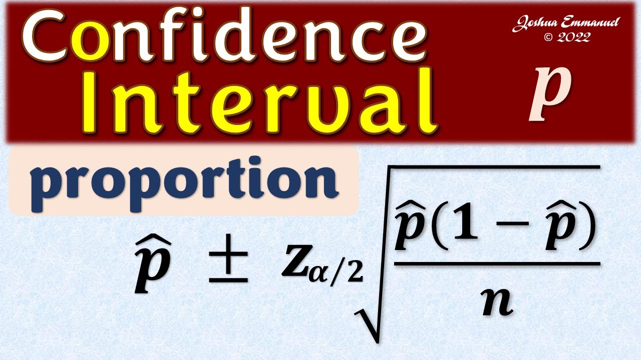
- 🔢 **Standard Error of Proportion**: The standard error for a sample proportion is calculated differently, using the formula SE = √(p(1-p)/n), where p is the sample proportion.
- 🌐 **Z-Statistic**: For proportions, the Z-statistic from the standard normal distribution is used when calculating confidence intervals, especially when the sample size is large.
- ✅ **Practical Application**: Understanding standard error and confidence intervals is crucial for making inferences about population parameters from sample data.
- 🤔 **Challenge Question**: The video concludes with a challenge question about determining how many additional measurements are needed to achieve a desired standard error, encouraging further discussion and deeper understanding.
Q & A
What is the standard error of the sample mean?
-The standard error of the sample mean, often abbreviated as SE, is a measure of the variability of the sample mean. It's calculated as the standard deviation (s) divided by the square root of the sample size (n), or SE = s / √n. It represents the uncertainty associated with the estimate of the population mean.
Why is the standard error important in statistics?
-The standard error is important because it indicates the precision of the sample mean as an estimate of the population mean. A smaller standard error means that the sample mean is likely to be closer to the population mean, which increases confidence in the estimate.
How does the sample size affect the standard error of the sample mean?
-As the sample size (n) increases, the standard error of the sample mean decreases. This is because the square root of n is in the denominator of the standard error formula, meaning that larger sample sizes lead to less variability and more precise estimates.
What is a confidence interval and how is it related to the standard error?
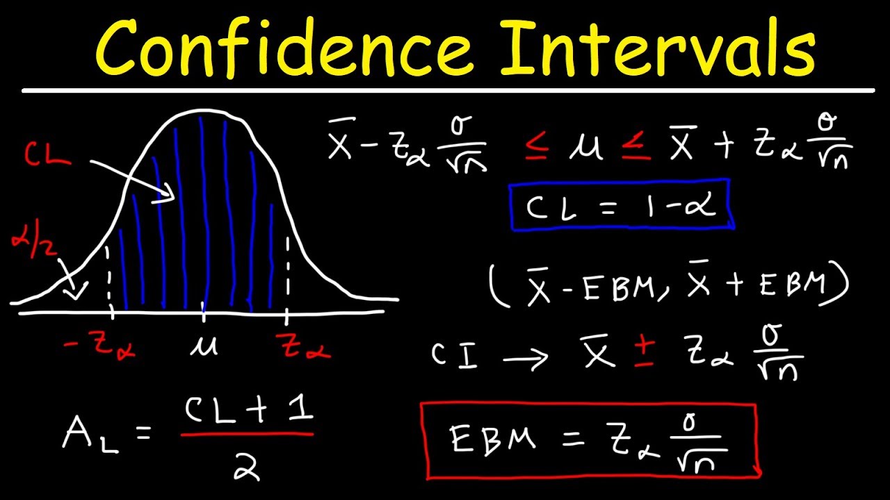
-A confidence interval is a range within which we expect the population parameter (like the population mean) to lie, with a certain level of confidence (e.g., 95%). It is calculated using the sample mean, the standard error, and a critical value from the appropriate distribution (like the t-distribution or the standard normal distribution).
What is the formula for the standard error of the sample proportion?
-The standard error of the sample proportion is calculated using the formula SE_p = √(p(1 - p) / n), where p is the sample proportion, and n is the sample size.
How does the central limit theorem apply to the sample proportion?
-The central limit theorem states that given a large enough sample size, the distribution of the sample proportions will approximate a normal distribution, regardless of the shape of the population distribution. This allows us to use the standard normal distribution for calculating confidence intervals for proportions when the sample size is large.
What is the difference between the standard error of the sample mean and the standard error of the sample proportion?
-The standard error of the sample mean is calculated using the standard deviation of the entire sample, while the standard error of the sample proportion is based on the variance of the proportion, which is p(1 - p) where p is the sample proportion. The sample mean's standard error is used for numerical data, whereas the sample proportion's standard error is used for categorical data.
Why might the confidence interval for a sample proportion be wider than expected?
-The confidence interval for a sample proportion can be wider than expected because it reflects the variability in the proportion, which can be quite large when dealing with categorical data (e.g., yes/no responses). Each observation contributes less information compared to numerical data, leading to wider intervals when the sample size is not very large.
How can you calculate the required sample size to achieve a desired standard error?
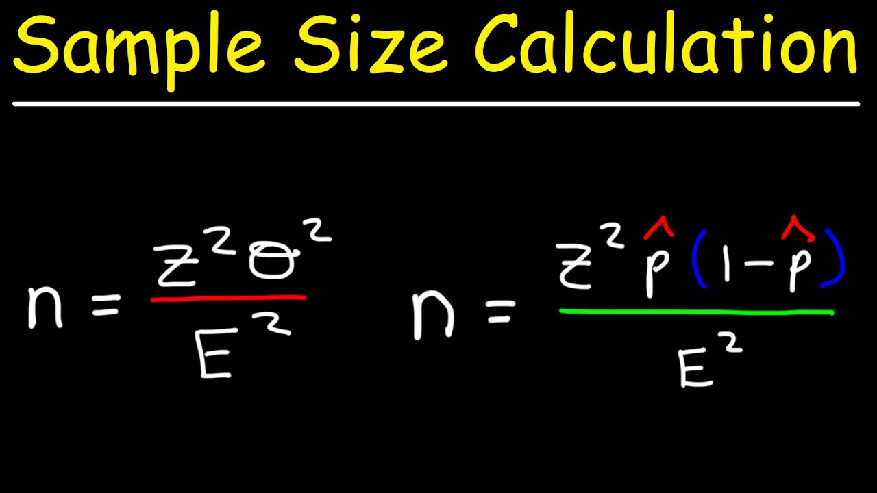
-To calculate the required sample size for a desired standard error, you would rearrange the standard error formula to solve for n. The formula would be n = s^2 / (SE desired)^2, where s is the known standard deviation of the population and SE desired is the standard error you wish to achieve.
What is the assumption required for using the t-distribution in calculating confidence intervals?
-The assumption required for using the t-distribution in calculating confidence intervals is that the population is normally distributed. However, for moderate to large sample sizes, the central limit theorem allows us to use the t-distribution even when the population distribution is not perfectly normal.
What is the challenge question posed in the video?
-The challenge question is to determine how many additional measurements are required to achieve a desired standard error, given a sample of 20 measurements with a noted sample mean and standard error.
Outlines
📊 Introduction to Standard Error of the Sample Mean
This paragraph introduces the concept of standard error, specifically the standard error of the sample mean. It's not typically categorized under descriptive statistics but is included in Microsoft Excel's descriptive stats package. The speaker aims to bridge basic descriptive measures with more advanced statistics. The standard error of the sample mean is defined and differentiated from standard deviation. A formula is provided, showing that it's derived from the standard deviation and the square root of the sample size (n). The concept is further explained with an example involving the average IQ of statistics students with varying sample sizes to illustrate how the standard error decreases as the sample size increases, leading to more confidence in the sample mean as an estimate of the population mean.
🔍 Understanding the Standard Error and Confidence Intervals
The second paragraph delves into the standard error as a measure of uncertainty in the sample mean. It explains that a higher standard error indicates more uncertainty and less confidence in the estimate of the true population mean. The relationship between the number of observations (n) and the standard error is clarified, with the standard error decreasing as n increases. The concept of confidence intervals is introduced, which are intervals within which we expect the population mean to lie with a certain level of confidence (e.g., 95%). The paragraph outlines the process of constructing a confidence interval using the sample mean, standard error, and a value from the T-distribution, which corresponds to the desired confidence level. The T-distribution is chosen based on the assumption that the population is normally distributed, which is a reasonable assumption for IQ scores.
📉 Calculating Confidence Intervals and Dealing with Proportions
The third paragraph focuses on calculating confidence intervals, specifically addressing the challenge of interpreting the distribution when dealing with proportions. It explains that while the sample mean is straightforward to calculate, finding the point on the T-distribution that corresponds to 97.5% of the distribution is less intuitive. The paragraph demonstrates how to use Excel's functions to find this point and calculate the confidence interval. It also discusses the difference in confidence intervals between different sample sizes and introduces the concept of the standard error of the sample proportion. An example is provided, where 65 out of 100 voters support a major party, to illustrate how to calculate the standard error of the sample proportion and construct a 95% confidence interval using the Z statistic from the standard normal distribution.
🎯 Central Limit Theorem and the Challenge Question
The final paragraph discusses the central limit theorem, which states that as the sample size (n) becomes large, the distribution of the sample proportion approaches a normal distribution, even if the underlying data is categorical. This allows for the use of the standard normal distribution (Z statistic) in calculating confidence intervals for proportions. The speaker then poses a challenge question, asking how many additional measurements would be needed to achieve a desired standard error, given a sample mean and standard error from a sample of 20 measurements. The paragraph concludes by encouraging further study and discussion on the topic and promoting the speaker's next video on sampling, which is linked in the video description.
Mindmap
Keywords
💡Standard Error
💡Sample Mean (X-bar)
💡Confidence Interval
💡Population Mean (MU)
💡Standard Deviation
💡Sample Size (n)
💡T-distribution
💡Central Limit Theorem
💡Z-statistic
💡Binomial Distribution
💡Degrees of Freedom
Highlights
This is the final video in the descriptive statistics series, focusing on standard error of the sample mean.
Standard error is a bridge between basic descriptive measures and more advanced statistics.
The standard error of the sample mean is calculated as the standard deviation divided by the square root of the sample size (s/√n).
As the sample size increases, the standard error decreases, leading to more confidence in the sample mean as an estimate of the population mean.
Confidence intervals can be constructed using the sample mean and the standard error, with a common interval being 95%.
The T distribution is used for calculating confidence intervals when the population standard deviation is unknown.
The central limit theorem states that as sample size increases, the sampling distribution of the sample mean approaches a normal distribution, regardless of the population distribution.
The standard error of the sample proportion is calculated using the formula √[p(1-p)/n], where p is the sample proportion.
For large sample sizes, the sample proportion is normally distributed, allowing the use of Z-statistics for confidence intervals.
The width of the confidence interval for proportions can be wider than expected, especially with categorical data.
The challenge question involves calculating how many more measurements are needed to achieve a desired standard error.
The video concludes with an invitation to subscribe for more statistical insights and to engage in discussion on the challenge question.
Excel's TINV and NORM.S.INV functions are used to find points on the T and standard normal distributions, respectively.
The video provides a practical example of calculating the standard error and confidence intervals using IQ test scores of different sample sizes.
The importance of the number of observations (n) in determining the precision of the sample mean as an estimate of the population mean is emphasized.
The video explains the concept of standard error in the context of Microsoft Excel's descriptive statistics output.
A comparison is made between the standard deviation and the standard error, highlighting their different roles in statistical analysis.
The video offers a challenge question to stimulate discussion and further exploration of statistical concepts among viewers.
The presenter, Justin Seltzer, encourages viewers to engage with the content by subscribing to the channel and leaving comments.
Transcripts
Browse More Related Video
Confidence Interval for a population proportion | Solved Problems
7.2.0 Estimating a Population Mean - Lesson Overview, Key Concepts, Learning Outcomes
How To Calculate The Sample Size Given The Confidence Level & Margin of Error
How To Find The Z Score, Confidence Interval, and Margin of Error for a Population Mean
Statistics 101: Confidence Intervals, Estimating Sample Size Needed
Statistics: Populations & Samples and Parameters vs Statistics
5.0 / 5 (0 votes)
Thanks for rating: