Calculus 2 Lecture 8.1: Solving First Order Differential Equations By Separation of Variables
TLDRThe video script offers an in-depth introduction to differential equations, focusing on their applications in various engineering fields. It explains the concept of order in differential equations and demonstrates how to solve first-order differential equations using integration. The instructor provides a clear example to illustrate the process of verifying a solution and discusses the general solution with an arbitrary constant. The script also covers separable differential equations, natural growth and decay models, and the law of cooling, providing practical examples such as bacterial growth and substance decay, and concludes with the calculation of cooling time for a turkey.
Takeaways
- 📚 The script is an educational introduction to differential equations, focusing on their applications in various engineering fields.
- 🔍 It emphasizes the importance of understanding the order of differential equations, which is the highest derivative present in the equation.
- 📈 The concept of separable differential equations is introduced as the simplest type, where the equation can be written as a product of two functions, one in terms of x and the other in terms of y.
- 📝 The script provides a step-by-step example of how to check if a given function is a solution to a differential equation by taking the derivative and comparing it to the original equation.
- 🔑 The role of arbitrary constants in general solutions of differential equations is explained, highlighting that they represent a family of curves.
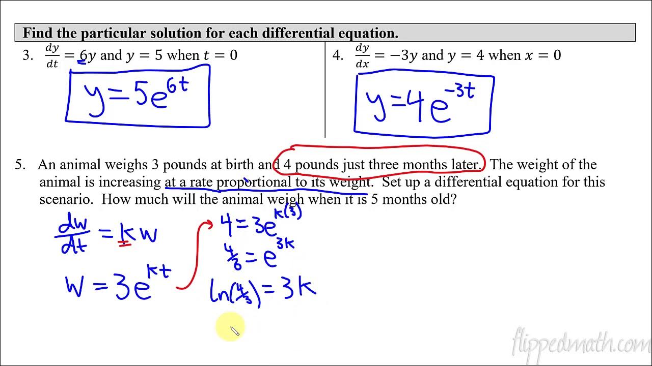
- 📌 The difference between general and particular solutions is clarified, with particular solutions arising from specific initial conditions that define a unique curve.
- 🧩 The process of solving separable differential equations involves separating variables, integrating both sides, and solving for the arbitrary constant using initial conditions.
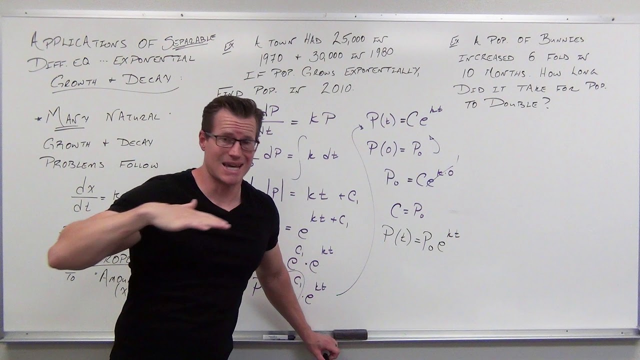
- 🌱 An example of natural growth or decay is presented, showing how to model population growth or substance decay using differential equations with an initial value.
- ⏱ The script discusses the law of cooling, which describes how the rate of cooling of an object is proportional to the temperature difference between the object and its surroundings.
- 🍪 A practical application of the law of cooling is given, using the example of cooling a turkey to determine the temperature at different times and when it would be safe to cut without burning fingers.
Q & A
What is the main topic discussed in the script?
-The main topic discussed in the script is differential equations, with a focus on first-order differential equations, separable differential equations, and their applications in various fields such as engineering and natural growth or decay models.
What is a differential equation of the first order?
-A first-order differential equation is an equation that involves a function and its first derivative. It is called 'first-order' because it contains only the first derivative of the function.
What does the 'order' of a differential equation signify?
-The 'order' of a differential equation signifies the highest derivative that occurs in the equation. For example, a first-order differential equation contains only the first derivative of the function.
What is a separable differential equation?
-A separable differential equation is a first-order differential equation that can be written as a product of two functions, one in terms of the independent variable (usually x) and the other in terms of the dependent variable (usually y).
How can you check if a function is a solution to a differential equation?
-To check if a function is a solution to a differential equation, you can differentiate the function with respect to the independent variable and see if it matches the right-hand side of the differential equation. If it does, the function is a solution.
What is the general solution of a first-order differential equation?
-The general solution of a first-order differential equation is a solution that contains an arbitrary constant, which represents the family of all possible solutions to the equation.
What is the difference between a general solution and a particular solution in the context of differential equations?
-A general solution includes an arbitrary constant and represents a family of curves or solutions that satisfy the differential equation. A particular solution, on the other hand, is a specific curve from that family, determined by an initial condition that assigns a specific value to the function and its derivative at a given point.
What is an initial condition in the context of differential equations?
-An initial condition is a specific value or set of values that is used to determine the particular solution of a differential equation. It typically specifies the value of the function and/or its derivative at a particular point in the domain.
How can the concept of natural growth or decay be modeled using differential equations?
-Natural growth or decay can be modeled using differential equations by assuming that the rate of change of a population or quantity is proportional to its current size. This leads to a first-order differential equation where the derivative of the quantity with respect to time is equal to a constant times the quantity itself.
What is the law of cooling and how is it related to differential equations?
-The law of cooling states that the rate of cooling of an object is proportional to the difference between its own temperature and the ambient temperature. This can be formulated as a first-order differential equation, where the temperature of the object over time can be modeled by solving the equation with appropriate initial conditions.
Outlines
📚 Introduction to Differential Equations
The speaker introduces the topic of differential equations, clarifying that the session will not be a comprehensive class on the subject but a basic introduction. They discuss the relevance of differential equations in engineering and various applications, emphasizing the importance of understanding the concept of 'order' in differential equations. The speaker also explains the difference between differential equations with unknowns in the derivative and those with functions of the derivative, providing an example of a first-order differential equation and how it can be solved by integration.
🔍 Exploring Differential Equations with Functions of Both Variables
The speaker delves into first-order differential equations that involve functions of both variables, X and Y, and highlights the challenges they present. They introduce the concept of separable differential equations as a simpler subset of these equations, where the variables can be separated for easier solving. The speaker reassures the audience that despite the complex terminology, the process of solving separable differential equations is manageable and builds upon previously learned concepts.
📉 Understanding the Concept of Separable Differential Equations
The speaker explains what constitutes a separable differential equation, focusing on the ability to separate the variables into a product or a sum. They provide examples of both separable and non-separable differential equations, illustrating the distinction between those that can be solved using separation of variables and those that cannot. The speaker also discusses the process of solving separable differential equations by integrating both sides of the equation with respect to the same variable.
🌐 Solving Separable Differential Equations with Examples
The speaker provides a step-by-step guide on solving separable differential equations, starting with ensuring the equation fits the criteria of being separable. They demonstrate the process of moving all terms involving one variable to one side and integrating both sides with respect to that variable. The speaker uses an example involving the natural logarithm and exponential functions to illustrate the integration process and the simplification of the resulting equation.
📌 Applying Initial Conditions to Differential Equations
The speaker discusses the use of initial conditions in differential equations, explaining how they allow for the determination of the arbitrary constant in the general solution. They differentiate between a general solution, which is a family of curves, and a specific solution, which is a single curve that passes through a given point. The speaker demonstrates how to apply an initial condition to find the specific solution to a differential equation.
🧩 Solving Differential Equations with Initial Values
The speaker continues the discussion on solving differential equations with initial values, emphasizing the process of finding the specific solution by substituting the initial values into the general solution to solve for the arbitrary constant. They reiterate the importance of having a general solution to plug in the numbers and show how the initial value problem helps in narrowing down to a single curve from the family of curves represented by the general solution.
🌱 Introduction to Natural Growth and Decay Models
The speaker introduces the concept of natural growth and decay models, which describe the change in a population or quantity over time based on its current size. They explain that these models are based on the principle of proportional change, where the rate of change is directly proportional to the current state. The speaker sets the stage for solving differential equations related to growth and decay by separation of variables.
📈 Developing a Model for Natural Growth and Decay
The speaker develops a model for natural growth and decay by solving a first-order differential equation that represents the rate of change of a population. They demonstrate the process of separating variables and integrating both sides with respect to time. The resulting model is an exponential function that includes an arbitrary constant, which can be determined using an initial condition.
🔄 Solving for the Arbitrary Constant in Growth and Decay Models
The speaker explains how to use an initial condition to solve for the arbitrary constant in the growth and decay model. They emphasize that the arbitrary constant represents the starting population or initial amount of the substance, and by plugging in the initial condition, one can determine its specific value. The speaker also highlights the importance of understanding the context of the model, such as the difference between growth and decay scenarios.
🍪 The Law of Cooling and Its Applications
The speaker discusses the law of cooling, which describes how an object cools over time in relation to the ambient temperature. They provide a personal anecdote about Thanksgiving and how the law of cooling can be applied to understand the rate at which food cools. The speaker emphasizes the importance of understanding the difference between the object's temperature and the ambient temperature in the cooling process.
🌡 Calculating the Cooling of an Object Over Time
The speaker provides a detailed explanation of how to calculate the temperature of an object over time using the law of cooling. They discuss the differential equation that models this process and demonstrate the steps to solve it by separation of variables. The speaker then shows how to use initial conditions to find a particular solution to the differential equation, which can be used to predict the temperature of the object at any given time.
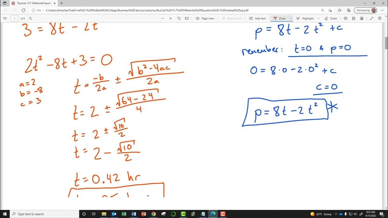
🕒 Determining the Time to Safely Cut the Turkey
The speaker concludes the discussion by addressing the practical question of how long one must wait to cut a turkey without burning their fingers. They use the particular solution derived from the law of cooling to calculate the time it takes for the turkey's temperature to drop to a safe level. The speaker demonstrates the process of plugging in the desired temperature into the model and solving for the time, providing a practical application of the concepts discussed.
Mindmap
Keywords
💡Differential Equations
💡Separable Differential Equations
💡Order of Differential Equation
💡Derivative
💡Integral
💡General Solution
💡Initial Value
💡Natural Growth and Decay
💡Half-Life
💡Law of Cooling
Highlights
Introduction to differential equations and their applications in various engineering fields.
Basic concept of differential equations, including the definition and order of the equation.
Explanation of first-order differential equations and how to solve them using integration.
The limitation of solving differential equations when the function is not solely in terms of X.
Introduction to separable differential equations and their simplicity in solving.
Demonstration of how to check if a function is a solution to a given differential equation.
The concept of general and specific solutions in differential equations.
Use of initial conditions to determine the specific solution from a general solution.
The process of solving separable differential equations by separating variables.
Integration techniques applied to both sides of a separable differential equation.
Handling of arbitrary constants during the integration of differential equations.
Solving a specific example of a separable differential equation step by step.
The use of natural logarithms and exponentiation to simplify solutions.
Addressing the concept of absolute value in the context of solutions to differential equations.
Combining logarithms and simplifying expressions within the solution process.
Interpretation of the solution to a differential equation in terms of growth or decay models.
Application of differential equations to model natural growth and decay processes.
Solving for the constant variation in a growth or decay model using given data points.
Using the model to predict future values based on the initial population or amount.
The relationship between the model of growth or decay and exponential functions.
Distinguishing between growth and decay based on the sign of the constant variation.
The invalidity of the model for non-proportional growth or decay scenarios.
Transcripts
Browse More Related Video

Calculus AB Homework 7.1 Differential Equations
Applications with Separable Equations (Differential Equations 14)
Calculus AB/BC – 7.8 Exponential Models with Differential Equations

AP Calculus AB - 7.8 Exponential Models With Differential Equations
BusCalc 13.7 Differential Equations

First order, Ordinary Differential Equations.
5.0 / 5 (0 votes)
Thanks for rating: