AP Calculus AB - 7.8 Exponential Models With Differential Equations
TLDRThe video script is a comprehensive lesson on exponential models using differential equations, presented by Mr. Bortnick for AP Calculus AB. It covers the basics of exponential functions, their growth or decay based on the value of the base 'b', and their applications in various scientific contexts like population growth and virus spread. The lesson delves into the calculus behind these models, including deriving the exponential function to find relationships between the rate of change and the size of the quantity. Mr. Bortnick guides through solving differential equations using separation of variables and emphasizes the general solution form for exponential growth and decay, which is y = c * e^(kt), where 'c' is the initial value and 'k' is a constant. The script also illustrates how to apply these models to real-world problems, such as predicting animal weight over time and calculating the doubling time of a population. The lesson concludes with an example of finding the value of 'k' for a population that doubles every seven years, reinforcing the concept of half-life and doubling time in exponential models.
Takeaways
- 📚 The lesson is about exponential models with differential equations, which are crucial in various scientific fields such as population growth and decay.
- 🧮 Students are advised to use a calculator and set it to radian mode, rounding to three decimal places for precision.
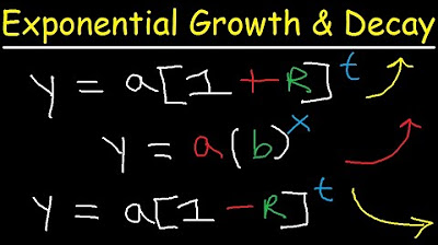
- 📈 The form of an exponential function is y = a * b^t, where 'a' is the initial value and 'b' is the growth or decay factor.
- 🔍 The growth or decay of an exponential function can be determined by the value of 'b': if b > 1, it's growth; if 0 < b < 1, it's decay.
- 📉 The derivative of an exponential function y = a * b^t with respect to time 't' results in dy/dt = a * b^t * ln(b), which simplifies to dy/dt = y * ln(b).
- 🌱 For exponential growth or decay problems, the differential equation is often in the form dy/dt = k * y, where 'k' is a constant.
- 🔑 The general solution to the differential equation dy/dt = k * y is y = c * e^(kt), where 'c' is the initial value and 'k' is the constant from the differential equation.
- 🦠 Exponential models are particularly useful in modeling scenarios such as animal weight gain, bacteria population changes, and radioactive decay.
- ⚖️ To find the specific solution for an exponential model, use the initial conditions to solve for the constants 'c' and 'k'.
- 📌 The concept of doubling time and half-life is directly related to exponential growth and decay, respectively, and is important in fields like biology and physics.
- 🧬 In the context of population growth, if a population doubles every 'n' years, the value of 'k' in the model can be found using the natural logarithm and the doubling period.
Q & A
What is the general form of an exponential function?
-The general form of an exponential function is y = a * b^t, where 'a' is the initial value, 'b' is the growth or decay factor, and 't' represents time.
How can you determine if an exponential function represents growth or decay?
-You can determine if an exponential function represents growth or decay by looking at the value of 'b'. If 'b' is greater than 1, it represents growth. If 'b' is less than 1 but greater than 0, it represents decay.
What is the derivative of the exponential function y = a * b^t with respect to time?
-The derivative of y with respect to time 't' is d(y)/dt = a * (natural log of b) * b^t.
What is the relationship between the rate of change of a quantity and its size in an exponential model?
-In an exponential model, the rate of change of a quantity is proportional to the size of the quantity. This means that the larger the quantity, the faster it grows, and the smaller it is, the slower it grows.
How can you solve the differential equation dy/dt = ky using separation of variables?
-To solve dy/dt = ky using separation of variables, you rearrange the equation to isolate y on one side, then integrate both sides. This results in the general solution y = c * e^(kt), where 'c' is the initial value of the model.
What is the significance of the constant 'k' in the differential equation dy/dt = ky?
-The constant 'k' in the differential equation dy/dt = ky determines the rate of growth or decay. If 'k' is positive, the function represents growth, and if 'k' is negative, it represents decay.
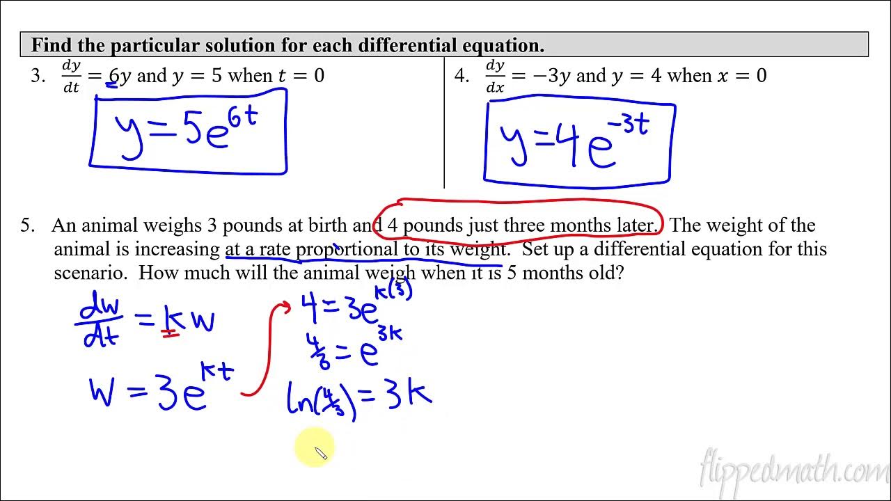
How can you find the particular solution to the differential equation dy/dt = 6y given that y = 5 when t = 0?
-To find the particular solution, you use the initial condition y = 5 when t = 0 to find the constant 'c' in the general solution y = c * e^(kt). Since dy/dt = 6y, 'k' is 6. Plugging in the values gives c = 5, and thus the particular solution is y = 5 * e^(6t).
What is the process to determine the weight of an animal at five months old given its weight at birth and three months later?
-First, set up a differential equation based on the information that the animal's weight increases at a rate proportional to its weight. Then, use the given weights at specific times to find the constants 'c' and 'k' in the general solution y = c * e^(kt). Finally, plug in the time value (t = 5 months) to predict the animal's weight.
How does the concept of half-life relate to exponential decay?
-Half-life is the time it takes for half of a substance undergoing exponential decay to decay away. It is a measure used particularly with radioactive materials and is directly derived from the exponential decay model.
What is the value of 'k' if a population doubles every seven years according to the model dy/dt = ky?
-To find the value of 'k', use the fact that the population doubles in seven years. This means that y = 2 when t = 7, given the initial condition y = 1 when t = 0. By substituting these values into the general solution y = c * e^(kt) and solving for 'k', you find that k = ln(2) / 7.
What is the role of the natural logarithm (ln) in solving exponential models?
-The natural logarithm (ln) is used to solve for the variable 'k' in the exponential model when the equation involves an exponential function of 'k'. By taking the natural log of both sides of the equation, you can eliminate the exponential and solve for 'k'.
Outlines
📚 Introduction to Exponential Models in Differential Equations
Mr. Bortnick introduces the topic of exponential models within the context of differential equations, specifically focusing on unit seven, topic 7.8. He emphasizes the need for a calculator and the importance of setting it to radian mode and rounding to three decimal places. The lesson begins with a review of exponential functions, discussing their applications in various contexts such as population growth, decay, and half-life. The variables 'a' and 'b' are defined, with 'a' representing the initial value and 'b' being the growth or decay factor. The instructor also explains how to determine whether an exponential function represents growth or decay by examining the value of 'b'.
🔢 Derivatives of Exponential Functions and Their Applications
The paragraph delves into the process of taking the derivative of an exponential function with respect to time, using implicit differentiation. It is shown that the derivative of an exponential function is a constant multiple of the original function, leading to the general form dy/dt = k*y. This form is crucial for recognizing exponential growth or decay, where the sign of the constant 'k' determines the nature of the process. The instructor then applies this understanding to various scenarios, such as the weight increase of an animal and the shrinking of a bacteria population, by setting up differential equations for each.
🧮 Solving Differential Equations Using Separation of Variables
This section covers the method of solving differential equations by separating variables. The instructor demonstrates how to rearrange the terms and integrate both sides of the equation to solve for 'y'. The solution to the differential equation dy/dt = ky is presented as y = c*e^(kt), where 'c' is the initial value and 'k' is the constant from the differential equation. The process is illustrated by solving a specific problem where dy/dt = 6y, with the initial condition y = 5 when t = 0. The solution is found by substituting the initial condition to find 'c' and using the coefficient from the differential equation as 'k'.
📈 Exponential Growth and Decay: Identifying 'c' and 'k'
The paragraph focuses on identifying the constants 'c' and 'k' in the general solution of an exponential model. It discusses how to use initial conditions to find the value of 'c' and how the coefficient from the differential equation represents 'k'. An example problem is solved, where the differential equation dy/dx = -3y is given, and the initial condition y = 4 when x = 0 is provided. The solution process involves substituting the initial condition to find 'c' and identifying 'k' from the differential equation.
🐾 Modeling Animal Weight Growth with Differential Equations
The paragraph presents a scenario where an animal's weight increases at a rate proportional to its current weight. The instructor sets up a differential equation for this scenario and uses given data points (the animal's weight at birth and three months later) to find the constants 'c' and 'k'. The process involves substituting the initial condition to find 'c', and then using another data point to solve for 'k'. The model is then used to predict the animal's weight at five months old, demonstrating the predictive power of exponential models.
📈 Understanding Growth and Decay in Exponential Functions
This section discusses the general form of exponential functions and how to identify whether they represent growth or decay. It explains that a positive exponent indicates growth, while a negative exponent indicates decay. The concept of doubling time and half-life is introduced, which are common applications of exponential models in various fields. A problem is solved to find the value of 'k' for a population that doubles every seven years, using the doubling time concept and the general solution of an exponential model.
🧠 Final Thoughts and Encouragement for Practice
The final paragraph wraps up the lesson with a summary of key points and an encouragement for students to practice the concepts learned. It emphasizes the importance of understanding the general form of exponential models and the ability to apply them to various problems. The instructor advises students to check their work and consult with their teacher if they have any questions, wishing them a great day ahead.
Mindmap
Keywords
💡Differential Equations
💡Exponential Functions
💡Growth and Decay
💡Initial Value
💡Growth or Decay Factor
💡Implicit Differentiation
💡Separation of Variables
💡Natural Logarithm
💡Exponential Growth/Decay Model
💡Half-Life
💡Doubling Time
Highlights
The lesson covers exponential models with differential equations, specifically focusing on how exponential functions can be used to model growth and decay.
Emphasizes the importance of setting calculators to radian mode and rounding to three decimal places for AP Calculus AB.
Exponential functions are introduced in the form of y = a * b^t, where 'a' is the initial value and 'b' is the growth or decay factor.
The derivative of an exponential function y = a * b^t with respect to time 't' is shown to be dy/dt = a * ln(b) * b^t, which simplifies to dy/dt = y * ln(b).
Discusses how the sign of the constant 'k' in the derivative dy/dt = k * y determines whether the function represents growth (k > 0) or decay (k < 0).
The concept that the rate of change of a quantity is proportional to the size of the quantity is central to exponential models.
Three scenarios are presented to demonstrate setting up differential equations for exponential growth and decay problems.
A method for solving differential equations of the form dy/dt = k * y using separation of variables is explained.
The general solution to dy/dt = k * y is given as y = c * e^(kt), where 'c' is the initial value of the model.
An example is worked through where an animal's weight is increasing exponentially, and the differential equation is used to predict future weights.
The concept of doubling time and half-life is introduced as a common application of exponential models in fields like biology and physics.
A problem involving a population that doubles every seven years is solved to find the value of the constant 'k' in the differential equation.
The lesson concludes with the practical application of exponential models in predicting future values based on current data points.
The importance of memorizing the general solution form y = c * e^(kt) for exponential models is highlighted for its frequent use in AP Physics and Calculus.
The process of using initial conditions to find the constants 'c' and 'k' in an exponential model is demonstrated through several examples.
The lesson provides a shortcut for recognizing and solving exponential models without needing to separate variables or take anti-derivatives.
The mathematical process of taking the natural log to solve for the constant 'k' in an exponential model is shown.
The practical use of exponential models in predicting the weight of an animal at different ages is demonstrated through a step-by-step calculation.
Transcripts
Browse More Related Video
Calculus AB/BC – 7.8 Exponential Models with Differential Equations
AP Calculus BC Lesson 7.9

Exponential Growth and Decay (Precalculus - College Algebra 66)
Modeling population with simple differential equation | Khan Academy
Calculus BC – 7.9 Logistic Models with Differential Equations
Exponential Growth and Decay Word Problems & Functions - Algebra & Precalculus
5.0 / 5 (0 votes)
Thanks for rating: