Calculus AB Homework 7.1 Differential Equations
TLDRThis educational video tutorial covers the solution of various calculus problems, focusing on differential equations and their applications. It demonstrates the process of finding derivatives, solving for particular solutions using initial conditions, and applying Newton's law of cooling. The script also explores exponential growth and decay, as well as the modeling of real-world scenarios such as bacterial growth and the cooling of an object, providing step-by-step solutions to engage viewers in advanced mathematical concepts.
Takeaways
- 📚 The video covers Unit 7 homework problems 1 through 12, focusing on differentiable functions and solving differential equations.
- 🔍 For problem 1, the function's first derivative is given as dy/dx = y^2 * 6 - 2x, and the task is to find and evaluate the second derivative at the point (3, 1/4).
- 📈 The second derivative d²y/dx² is found using the product rule and chain rule, resulting in a calculation that evaluates to -1/8 at the specified point.
- 🧩 In Part B, the video solves a differential equation dy/dx = y^2 * 6 - 2x with an initial condition to find the function y = f(x).
- 🔑 The solution to the differential equation involves separating variables and integrating both sides to find the general solution for y in terms of x and a constant C.
- 📉 For a horizontal tangent line problem, the video demonstrates using the second derivative test to determine the concavity and local extrema of a function.
- 🌟 The video explains the process of solving differential equations with initial conditions, such as finding the particular solution for y = f(x) when given f(3) = 1/4.
- 🚧 An example of a real-world application is given, where the rate of oil pumping is proportional to the amount of oil left in the well, leading to an exponential decay model.
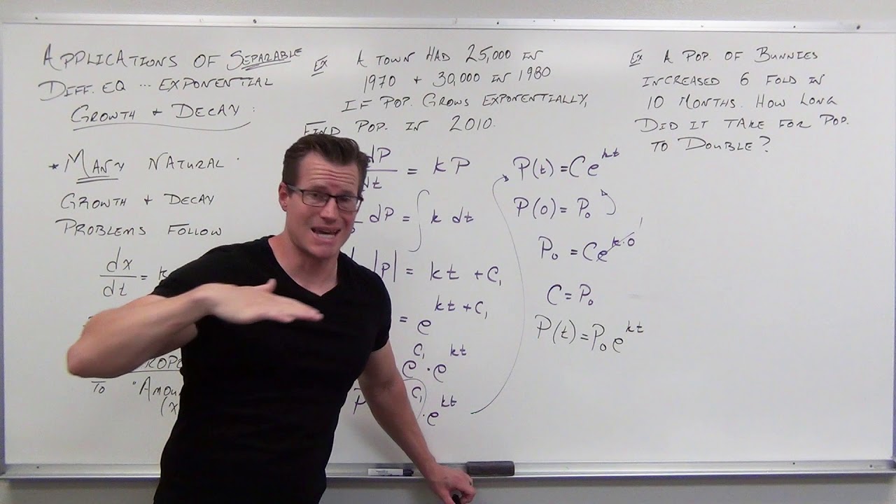
- ⏳ The script discusses the use of differential equations to model population growth, such as the number of wolves or bacteria, with rates proportional to the current population size.
- 🌡 The video also covers Newton's law of cooling, which is a differential equation that models the cooling process of an object in a surrounding environment.
- 📊 Finally, the script touches on various other differential equations, including those modeling the surface area change of a cube and bacterial population growth over time.
Q & A
What is the first derivative of the function given by dy/dx = y^2 * 6 - 2x?
-The first derivative is already given in the script as dy/dx = y^2 * 6 - 2x. This represents the slope of the tangent to the graph of y = f(x) at any point (x, y).
How do you find the second derivative d^2y/dx^2 of the function mentioned in the script?
-To find the second derivative, you differentiate the first derivative with respect to x, using the product rule and chain rule as shown in the script. The result is 2y * dy/dx - 2.
What is the value of the second derivative at the point (3, 1/4)?
-After evaluating the first derivative at the point (3, 1/4) and substituting it into the second derivative formula, the value is found to be -1/8.
How can you solve the differential equation dy/dx = y^2 * 6 - 2x with the initial condition f(3) = 1/4?
-You separate variables and integrate both sides of the equation. The general solution is found to be y = 1/(x^2 - 6x + C). Using the initial condition, you can solve for C and get the particular solution.
What is the process to find the x-coordinate of the point of tangency for the horizontal line y = -2?
-Since the slope of a horizontal line is 0, you set dy/dx to 0 and solve for x, which gives x = 3. The point of tangency is therefore at (3, -2).
How do you determine if the function has a local maximum, local minimum, or neither at the point of tangency?
-You use the second derivative test. If the second derivative at the point is positive, the function is concave up, indicating a local minimum at that point.
What is the differential equation for the amount of oil being pumped from a well, and how is it solved?
-The differential equation is dy/dt = K * y, where y is the amount of oil and K is the constant of proportionality. It is solved by separating variables and integrating both sides.
How do you find the particular solution for the oil pumping problem given certain initial conditions?
-You use the initial conditions to solve for the constant K in the general solution. Then, you substitute the value of K back into the general solution to get the particular solution.
What is the rate of change of the amount of oil in the well when there are 600,000 gallons remaining?
-You use the derivative of the particular solution for y (the amount of oil) with respect to time t, which is dy/dt = K * y. Substituting y with 600,000 gives the rate of change at that moment.
How do you determine the time when it is no longer profitable to pump oil from the well?
-You solve the inequality set up by the condition that there are fewer than 50,000 gallons remaining, using the particular solution for y in terms of t. The solution gives the time t when pumping should stop.
Outlines
📚 Calculus Homework - Unit 7 Problems 1-12
This paragraph introduces a calculus homework session covering unit 7 problems 1 through 12. The focus is on a function 'f' that is differentiable for all real numbers, with a specific interest in the slope of the graph at the point (3, 1/4). The derivative at any point (x, y) is given by dy/dx = y^2 * 6 - 2x. Part A of the problem requires finding the second derivative and evaluating it at the specified point, while Part B involves solving a differential equation with an initial condition to find the function 'y = f(x)'.
🔍 Analyzing the Second Derivative and Solving Differential Equations
The speaker delves into the process of finding the second derivative of the given function, applying the product rule and chain rule where necessary. After calculating the second derivative, they evaluate it at the point (3, 1/4) and find it to be -1/8. Moving on to Part B, they solve a differential equation to find 'y = f(x)', using separation of variables and integration to arrive at the general solution. An initial condition is applied to find the particular solution and the value of the constant 'C' in the equation.
🌐 Differential Equations with Initial Conditions and Tangency Points
The paragraph discusses solving differential equations with given initial conditions and finding points of tangency. The speaker first solves a differential equation to find the function 'y = f(x)' and then applies an initial condition to determine the constant 'C'. They then consider a new differential equation and use the condition that the slope is zero at a point of tangency to find the x-coordinate of the tangency point. A second derivative test is performed to determine the nature of the critical point found.
📉 Exponential Decay of Oil Extraction
This section models the exponential decay of oil being pumped from a well, with the rate of extraction proportional to the amount of oil left. The speaker sets up a differential equation for the situation and solves it using separation of variables and integration. Initial and boundary conditions are applied to find the specific values of the constant 'K' and to determine when it is no longer profitable to pump oil from the well.
🐺 Population Dynamics of a Wolf Pack
The paragraph examines the population dynamics of a wolf pack, where the rate of increase is proportional to the current population size. The speaker translates this into a differential equation and solves it using separation of variables and integration techniques. Initial conditions are used to find the particular solution for the population over time, and a second data point is applied to determine the constant of proportionality 'K'.
🍲 Newton's Law of Cooling and its Application
The speaker discusses Newton's law of cooling, which describes the rate at which an object cools in relation to its surroundings. They set up a differential equation based on this law and solve it by separating variables and integrating. Initial conditions are used to find the specific form of the solution, and an example is given to find the time it takes for the temperature of an object to reach a certain value.
🕵️♂️ Using Newton's Law to Solve a Murder Case
In this paragraph, the speaker applies Newton's law of cooling to a murder investigation scenario. They establish a differential equation based on the temperature change of a body and solve it to estimate the time of death. Initial and boundary conditions are used to find the constant 'K' and to calculate the time when the victim's body temperature was at a normal level.
🧬 Bacterial Growth Model Using Differential Equations
The speaker presents a model for the growth of a bacterial population, which is described by a differential equation where the rate of growth is proportional to the current population size. They solve the differential equation using separation of variables and integration. Initial conditions and a doubling condition are applied to find the constant 'K' and to determine the factor by which the population has increased over time.
🦆 Modeling Duckling Growth with Differential Equations
This section discusses the growth of a duckling's weight over time, modeled by a differential equation where the rate of weight increase is proportional to the current weight. The speaker solves the differential equation and uses initial conditions to find the particular solution for the duckling's weight. They then calculate the weight of the duckling at a future time point, six months after hatching.
📏 Rate of Change of a Cube's Surface Area
The speaker introduces a problem involving the rate of change of a cube's surface area with respect to time, which is directly proportional to the square root of a fraction of the surface area. They write a differential equation to model this relationship, setting the foundation for further analysis or solution of the problem.
🦠 Bacterial Population Growth Over Three Days
In this paragraph, the speaker examines the growth of a bacterial population over the first three days, with the rate of growth proportional to the current population size. They solve the differential equation using separation of variables and integration, apply initial conditions to find the constant 'K', and calculate the population size on the third day. They conclude by determining the factor by which the population has increased over the three-day period.
Mindmap
Keywords
💡Differentiable
💡First Derivative
💡Second Derivative
💡Differential Equation
💡Product Rule
💡Chain Rule
💡Implicit Differentiation
💡Initial Condition
💡Separation of Variables
💡Integral
💡Newton's Law of Cooling
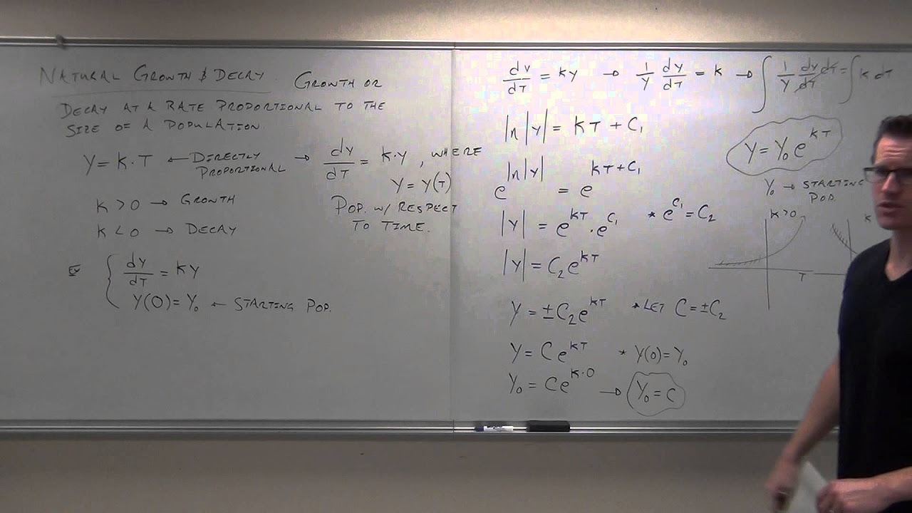
💡Exponential Growth/Decay
Highlights
The video covers unit 7 homework problems 1 through 12 involving calculus concepts.
Problem 1 introduces a differentiable function f for all real numbers with a specific point on its graph and a given slope formula dy/dx = y^2 * 6 - 2x.
Part A of the problem requires finding the second derivative d^2y/dx^2 using the product rule and evaluating it at a given point.
The evaluation of the second derivative at the point (3, 1/4) results in a value of -1/8.
Part B involves solving a differential equation with an initial condition to find the function y = f(x).
The differential equation is solved by separating variables and integrating both sides.
A general solution for y in terms of x is obtained, which is then particularized using an initial condition.
The final solution for y as a function of x is provided.
Problem 2 explores the concept of a tangent line to a graph and the conditions for a local maximum or minimum using the first and second derivatives.
The x-coordinate of the point of tangency is found to be 3, with the line y = -2 being tangent to the graph.
A second derivative test confirms the presence of a local minimum at the point of tangency.
Problem 3 models the rate of oil pumping from a well, which is proportional to the amount of oil left.
An equation for the amount of oil remaining in the well at any time T is derived and solved using initial conditions.
The rate at which the amount of oil in the well is decreasing is calculated when 600,000 gallons remain.
The time at which it is no longer profitable to pump oil is determined to be when less than 50,000 gallons remain.
The video concludes with a problem involving the population growth of wolves, modeled by a differential equation.
The population P of T is expressed in terms of T and K, with an initial condition of 500 wolves.
The video demonstrates the process of solving differential equations with various initial conditions and real-world applications.
Transcripts
Browse More Related Video

Calculus 2 Lecture 8.1: Solving First Order Differential Equations By Separation of Variables

Applications with Separable Equations (Differential Equations 14)

Exponential Growth and Decay (Precalculus - College Algebra 66)

Differential Equations with Velocity and Acceleration (Differential Equations 7)

Math 11- Section 2.6 (previously section 3.5)

AP Calculus AB - 7.8 Exponential Models With Differential Equations
5.0 / 5 (0 votes)
Thanks for rating: