Diagonalization
TLDRThe video explains the process of matrix diagonalization, which involves writing a matrix A as the product of two matrices X and D, where D is a diagonal matrix containing the eigenvalues of A. By rearranging terms, the equation X−1AX=D shows that multiplying A by eigenvector matrix X diagonalizes it. The steps are: 1) Find A's eigenvalues/vectors, 2) Build diagonal matrix D from eigenvalues, 3) Build matrix X from corresponding eigenvectors, 4) Invert X and multiply all matrices to verify you get A. Diagonalization simplifies matrix computations and is valuable technique.
Takeaways
- 😃 Diagonalization involves writing a matrix A as XDX−1, where D is a diagonal matrix. This makes computations easier.
- 😊 X is made up of A's eigenvectors and D is made up of A's eigenvalues. The order must match between X and D.
- 🤓 To diagonalize A, first find its eigenvalues and corresponding eigenvectors.
- 😎 The diagonal terms of D are the eigenvalues, ordered consistently with the eigenvector columns of X.
- 🧐 The process only works if A has distinct eigenvalues or independent eigenvectors for duplicate eigenvalues.
- 👍 Once the eigenvalues and eigenvectors are found, constructing D and X is straightforward.
- 🤔 Multiplying XDX−1 should give back the original matrix A, as a check.
- 🤯 Diagonalization makes matrix computations more efficient and computer-friendly.
- 😮 The inverse of X is needed to recover A from its diagonalized form XDX−1.
- 😀 Check that A = XDX−1 by multiplying out the matrices to verify diagonalization worked.
Q & A
What is diagonalization?
-Diagonalization is the process of taking a matrix and writing it as the product of two matrices, one of which is a diagonal matrix. It involves finding the eigenvalues and eigenvectors of the original matrix.
When can a matrix be diagonalized?
-A matrix can be diagonalized if it has n distinct eigenvalues, or if it has repeated eigenvalues, there must exist n linearly independent eigenvectors associated with those eigenvalues.
How is the diagonal matrix D constructed in the diagonalization process?
-The diagonal matrix D contains the eigenvalues of the original matrix along its diagonal, in the same order as the eigenvectors in the matrix X.
How is the matrix X constructed in the diagonalization process?
-The matrix X has the eigenvectors of the original matrix as its columns, in the same order as the corresponding eigenvalues in the diagonal matrix D.
Why is consistency in ordering important when constructing the matrices?
-The order of the eigenvalues in D must match the order of the corresponding eigenvectors in the columns of X. The first column of X matches the first diagonal entry of D, etc.
What was the purpose of verifying the matrix multiplication at the end?
-Multiplying the matrices X, D, and X-1 at the end and getting back the original matrix A verifies that the diagonalization process was done correctly.
What are the benefits of diagonalization?
-Diagonalization makes computations and analysis with matrices easier since a diagonal matrix is simpler. It also makes matrices more computer-friendly.
How do you find the inverse of the matrix X?
-For a 2x2 matrix, the inverse is found by swapping the diagonal entries, changing the sign of the off-diagonal entries, and dividing the whole matrix by the determinant.
What if a matrix does not have enough linearly independent eigenvectors?
-If a matrix does not have enough linearly independent eigenvectors for repeated eigenvalues, it cannot be fully diagonalized. We can diagonalize it as much as possible.
Can any matrix be converted into a diagonal matrix?
-No, only square matrices that have a complete set of linearly independent eigenvectors can be fully diagonalized into a diagonal matrix.
Outlines
📗 Introducing Matrix Diagonalization
This paragraph introduces the concept of matrix diagonalization, which involves writing a matrix A as a product of matrices X, D, and X^-1, where D is a diagonal matrix. This is possible when A has distinct eigenvalues with associated linearly independent eigenvectors. D contains the eigenvalues of A along its diagonal, while X contains the eigenvectors of A as columns ordered consistently with D. Diagonalization is useful because it simplifies computations and operations with matrices.
💻 Example of Matrix Diagonalization
This paragraph walks through an example of diagonalizing the 2x2 matrix A = [-3, -4; 5, 6]. The eigenvalues and eigenvectors of A are found, then used to construct the diagonal matrix D and matrix X. The inverse of X is also calculated. Finally, the product XDX^-1 is shown to reconstruct the original matrix A, verifying the diagonalization process.
Mindmap
Keywords
💡diagonalization
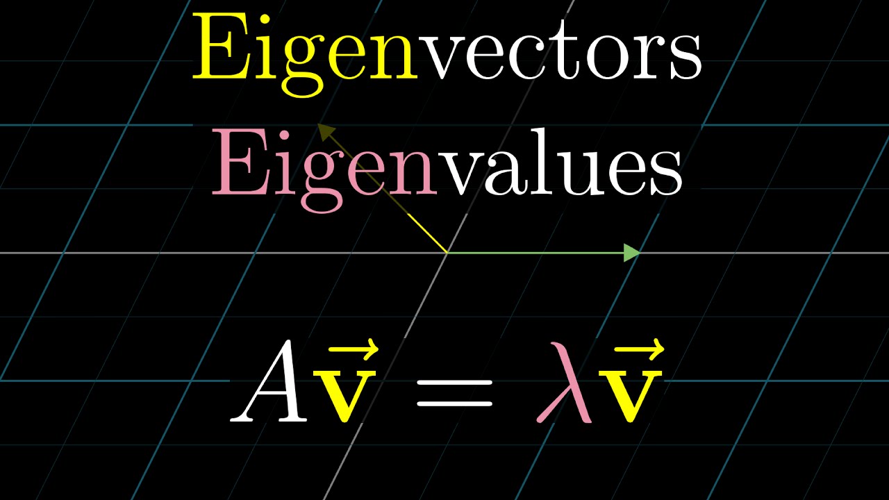
💡eigenvalues
💡eigenvectors
💡diagonal matrix
💡linearly independent
💡inverse
💡verification
💡computation
💡characteristic polynomial
💡linearly combine
Highlights
Diagonalization involves taking a matrix and writing it as a product of matrices, one of which only has values along the diagonal.
The X matrix is said to diagonalize A, because multiplying A in this way gives us the diagonal matrix D.
The reason for this is that the diagonal matrix D is simply made up of the eigenvalues of A, while the matrix X is made up of the eigenvectors.
Once we know the eigenvalues and eigenvectors of a matrix, the diagonalization process is easy.
The first column of the X matrix must be the eigenvector associated with the eigenvalue in the first term for the diagonal of D, same with the second column of X and the second term for the diagonal of D, and so on.
By factoring this we see that (λ - 1)(λ - 2) = 0, which means our solutions and eigenvalues are λ = 1 and λ = 2.
We don't have to worry about the second row here because it ends up giving us the same thing.
Now that we have all of our eigenvalues and eigenvectors, we can write out the diagonal matrix D and the matrix X.
The only remaining piece is the inverse of X. Since X is a 2 by 2 matrix, we simply swap the top left and bottom right elements, multiply the off-diagonal elements by -1, and divide the whole matrix by the determinant.
Diagonalization helps make computations with matrices much easier and computer friendly, making it a valuable process to remember.
First take D times X−1 and we get -5, -4; 10, 10.
Next we will multiply X by this new matrix, giving us 5 minus (4/5 times 10), 4 minus (4/5 times 10); -5 + 10, -4 + 10.
We end up with -3, -4; 5, 6, which was indeed the matrix A we started with.
Diagonalization helps make computations with matrices much easier and computer friendly,
so let’s check comprehension.
Transcripts
Browse More Related Video

21. Eigenvalues and Eigenvectors

Finding Eigenvalues and Eigenvectors
Eigenvectors and eigenvalues | Chapter 14, Essence of linear algebra

Matrix Multiplication and Associated Properties

PreCalculus - Matrices & Matrix Applications (21 of 33) Using the Determinant to Find the Inverse
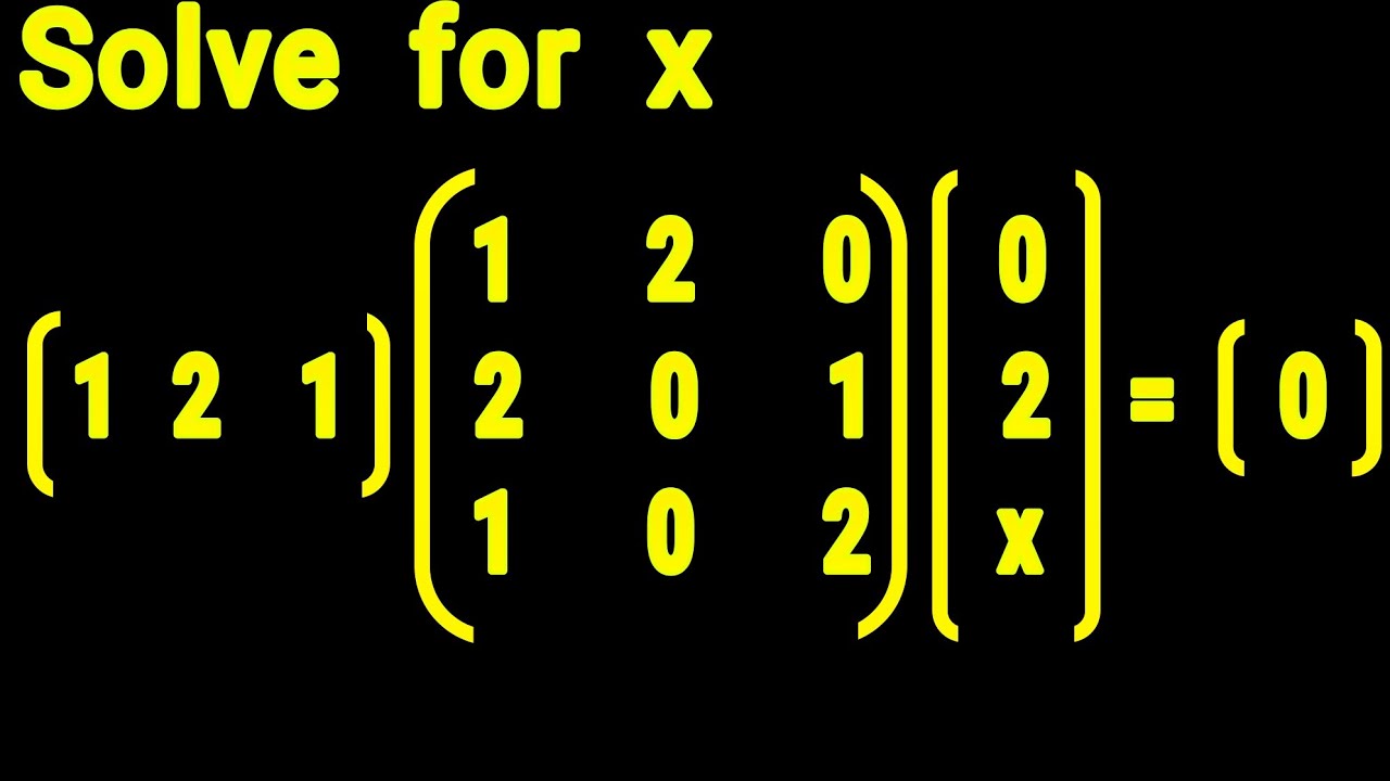
Solve for x | Matrix Multiplication
5.0 / 5 (0 votes)
Thanks for rating: