Calculus BC – 7.9 Logistic Models with Differential Equations
TLDRIn this engaging calculus lesson, Mr. Bean delves into the intricacies of logistic growth differential equations, a topic essential for the AP exam. The video begins with an introduction to logistic growth, illustrating it with a graph and explaining its real-world applications, such as population growth with animals or humans. The concept of a carrying capacity or limiting value is introduced, representing the maximum population size that an environment can sustain. The video highlights the importance of the point of inflection in logistic growth, where the growth rate transitions from increasing to decreasing. Mr. Bean then demonstrates how to recognize and manipulate logistic differential equations in two common forms. He emphasizes the significance of understanding the maximum value of the function and the maximum rate of change, which occurs at half the carrying capacity. The lesson progresses to solving differential equations and finding carrying capacities, with Mr. Bean guiding viewers through the process of separation of variables and partial fractions. The video concludes with a challenge to find a differential equation that represents a given situation, showcasing the practical application of logistic growth models. This comprehensive overview of logistic differential equations is both informative and accessible, making complex calculus concepts more digestible for students.
Takeaways
- 📈 The logistic growth model represents population growth that starts off exponential but slows down as it approaches a limiting value or carrying capacity.
- 🔍 The point of inflection in a logistic growth graph is a critical point where the growth rate changes from increasing to decreasing.
- 📌 The maximum growth rate of a logistic function occurs when the population size is half of the carrying capacity.
- 📘 Logistic differential equations can be written in two forms, and recognizing these forms is crucial for solving problems related to logistic growth.
- ✅ The carrying capacity (l) is the maximum value that the population can reach, and it is a key parameter in logistic growth models.
- 🤔 Distinguishing between the maximum value of the function (the carrying capacity) and the maximum rate of change is essential for understanding logistic growth.
- 🧮 To solve logistic differential equations, separation of variables and partial fraction decomposition are often used, leading to the standard form of a logistic function.
- ✋ Practice is key to recognizing the logistic form of a differential equation, which can save time in problem-solving as opposed to converting to standard form.
- 🔢 The value of k in a logistic differential equation can be determined by using given rates of change and population sizes.
- 📉 The logistic function's growth rate decreases after the point of inflection, which is a point of practical significance in modeling real-world scenarios like population growth.
- 🌐 Real-world applications of logistic growth include modeling animal populations and understanding the limits of human population growth on Earth.
Q & A
What is the main topic of the lesson?
-The main topic of the lesson is logistic growth differential equations and their application in calculus.
What is the logistic function's graph typically shaped like?
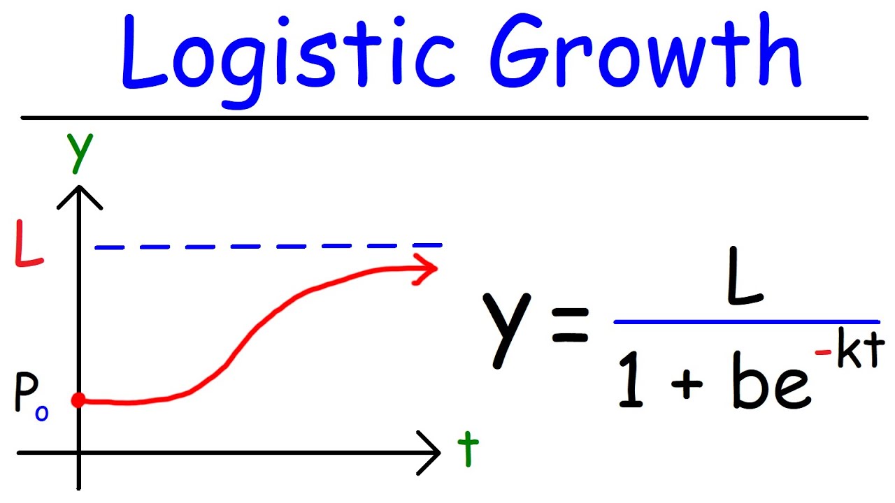
-The logistic function's graph starts small, grows almost exponentially, then slows down and reaches a cap or ceiling, which is known as the limiting value or carrying capacity.
What is the real-world application of logistic growth?
-A real-world application of logistic growth is population growth, such as animal populations or human beings on Earth, which cannot grow indefinitely due to limitations in carrying capacity.
What is the significance of the point of inflection in a logistic growth graph?
-The point of inflection is significant because it marks the transition point where the growth rate changes from increasing to decreasing. Before this point, the population grows faster and faster, and after this point, the growth rate slows down.
What is the general form of a logistic differential equation?
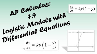
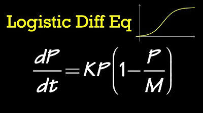
-A logistic differential equation can generally be written in two forms: k * y * (1 - y/l) or k * (l - y) / y, where k is a constant, y is the dependent variable, and l is the limiting value or carrying capacity.
At what y-value does the logistic function have its maximum growth rate?
-The maximum growth rate of a logistic function occurs when y equals l/2, which is half of the limiting value.
How can you identify a logistic differential equation in a problem?
-You can identify a logistic differential equation by recognizing the dependent variable y appearing twice and in the form of 1 - y/l or l - y, with l being the limiting value.
What is the maximum value of the logistic function?
-The maximum value of the logistic function is the limiting value (l), which represents the highest y-value that the function will reach.
What is the maximum rate of change in a logistic function?
-The maximum rate of change in a logistic function occurs at the point of inflection, which is when y equals half of the limiting value (l/2).
How can you solve a logistic differential equation to find the function y?
-To solve a logistic differential equation for y, you would separate variables, use partial fractions if necessary, and integrate to find the form of the logistic function, which typically involves the carrying capacity (l) and a constant k.
What is the carrying capacity in the context of logistic growth?
-The carrying capacity, often denoted as l, is the maximum population size that an environment can sustain indefinitely without being degraded, which is a key parameter in logistic growth models.
Outlines
📈 Introduction to Logistic Growth Differential Equations
The first paragraph introduces the topic of logistic growth differential equations, which are used to model population growth with a carrying capacity. The logistic function is represented graphically with a characteristic S-curve that starts with exponential growth, slows down, and then levels off at a maximum value known as the carrying capacity. The concept is applied to real-world scenarios like animal populations, emphasizing the impossibility of indefinite growth. The point of inflection, where the growth rate changes from increasing to decreasing, is highlighted as a critical value. The logistic differential equation is introduced in two common forms, emphasizing the importance of recognizing the dependent variable's appearance and the carrying capacity in the equation.
🔍 Analyzing Logistic Functions and Maximum Growth Rates
This paragraph delves into the specifics of logistic functions, focusing on how to identify and calculate the maximum value and the maximum rate of change. It explains that the maximum value of the function corresponds to the carrying capacity (l), while the maximum growth rate occurs at half of the carrying capacity (l/2). The paragraph provides examples of how to recognize the logistic form of a differential equation and how to solve for the dependent variable y in the general form of a logistic differential equation using separation of variables and partial fraction decomposition.
🧮 Solving Logistic Differential Equations with Given Conditions
The third paragraph demonstrates how to apply logistic differential equations to a scenario involving a state park with a known carrying capacity and current population. It guides through setting up the logistic differential equation using the given rate of change and solving for the unknown growth rate constant (k). The process involves substituting known values into the logistic equation, solving for k, and simplifying the equation to its standard logistic form. The paragraph also emphasizes the importance of practicing both forms of the logistic equation for better understanding and problem-solving.
🔑 Finding the Carrying Capacity from a Logistic Differential Equation
The final paragraph addresses the task of finding the carrying capacity (l) from a given logistic differential equation. It outlines a method to rearrange the equation into a form that makes the carrying capacity explicit. The process involves algebraic manipulation, including factoring and simplifying fractions, to express the equation in a form that clearly shows the carrying capacity. The paragraph concludes by encouraging mastery of logistic differential equations and looking forward to the next unit.
Mindmap
Keywords
💡Logistic Growth
💡Carrying Capacity
💡Point of Inflection
💡Exponential Growth
💡Differential Equation
💡Second Derivative Test
💡Separation of Variables
💡Partial Fractions
💡Maximum Growth Rate
💡Standard Form
💡Practice Problems
Highlights
Logistic growth differential equations are focused on in the calculus lesson.
Logistic growth has a ceiling or cap, known as the limiting value or carrying capacity.
The logistic function starts with exponential growth and then slows down to reach a cap.
A real-world application of logistic growth is population growth with animals or humans.
The point of inflection in a logistic growth graph is a critical value indicating the shift from accelerating to decelerating growth rate.
The growth rate increases until the point of inflection and decreases thereafter.
The logistic differential equation can be written in two forms, recognizing the dependent variable appearing twice is key.
The point of inflection occurs at y equals l/2, where l is the limiting value.
The maximum growth rate of a logistic function occurs when y is half of the limiting value.
The logistic differential equation involves the carrying capacity (l) and the growth rate (k).
The maximum value of the logistic function is the carrying capacity, and the maximum rate is when y equals l/2.
Differentiating between the maximum value and the maximum rate of change is crucial for solving logistic problems.
The general form of a logistic differential equation can be solved using separation of variables.
Partial fraction decomposition is used to integrate the separated equation and find the logistic function form.
When creating a logistic differential equation from a scenario, it's important to identify the carrying capacity and growth rate.
The carrying capacity can be found by manipulating the logistic equation into one of its standard forms.
Recognizing the two forms of logistic differential equations is essential for solving practice problems and exams.
The lesson concludes with a mastery check and a test, emphasizing the importance of understanding logistic growth models.
Transcripts

5.0 / 5 (0 votes)
Thanks for rating: