How to Calculate Market Equilibrium | (NO GRAPHING) | Think Econ
TLDRThis educational video teaches viewers how to algebraically determine equilibrium price and quantity in economics, without the need for graphical representation. The presenter uses two equations, one for quantity demanded and one for quantity supplied, and demonstrates the process of solving for the equilibrium price (P* = 16) and quantity (Q* = 52). The video simplifies the concept by showing how to equate the demand and supply equations and solve for the unknown variable, emphasizing the importance of distinguishing equilibrium values with an asterisk for clarity.
Takeaways
- 📚 The video teaches how to find equilibrium quantity and price without drawing supply and demand graphs.
- 🔢 The given supply and demand equations are Qd = 100 - 3P and Qs = 2P + 20, representing the inverse relationship between price and quantity demanded, and the direct relationship between price and quantity supplied.
- 📉 The law of demand is illustrated with a negative coefficient for P in the demand equation, showing that as price increases, quantity demanded decreases.
- 📈 The positive coefficient of P in the supply equation indicates that as price increases, quantity supplied also increases.
- ⚖️ Equilibrium is found where quantity demanded equals quantity supplied, which is the intersection of the demand and supply curves.
- 📝 Algebraic method is used to solve for equilibrium by setting Qd equal to Qs, resulting in a single equation with one unknown, P.
- 🧩 The process involves combining like terms and isolating P to find the equilibrium price, which in this case is P = 16.
- 🔑 Using the equilibrium price, the equilibrium quantity can be found by substituting P back into either the demand or supply equation, yielding Q = 52.
- 🔄 The video demonstrates substituting the equilibrium price into both the demand and supply equations to confirm the same equilibrium quantity is obtained.
- 📈 The equilibrium point is represented as (Q*, P*) = (52, 16), with an asterisk to denote equilibrium values and avoid confusion.
- 👍 The video encourages viewers to like, subscribe, and comment if they find the content helpful, emphasizing the educational value of the lesson.
Q & A
What is the main topic of the video?
-The video is about determining equilibrium quantity and price without drawing a supply and demand graph, using algebraic methods.
What is the relationship between price and quantity demanded as per the law of demand?
-According to the law of demand, there is an inverse relationship between price and quantity demanded, meaning as price goes up, quantity demanded goes down.
How is the relationship between price and quantity supplied represented in the video?
-The relationship between price and quantity supplied is represented as a positive correlation, meaning as price increases, quantity supplied also increases.
What are the equations for quantity demanded and quantity supplied given in the video?
-The equation for quantity demanded is Qd = 100 - 3P, and for quantity supplied, it is Qs = 2P + 20.
What does the equilibrium in economics mean in the context of this video?
-In the context of this video, equilibrium refers to the point where the quantity demanded equals the quantity supplied, which is where the demand and supply curves would intersect.
How does the video suggest finding the equilibrium price algebraically?
-The video suggests setting the quantity demanded equal to the quantity supplied (Qd = Qs) and solving the resulting equation for the price variable P.
What is the equilibrium price calculated in the video?
-The equilibrium price calculated in the video is P = 16.
How is the equilibrium quantity found using the equilibrium price?
-The equilibrium quantity is found by substituting the equilibrium price back into either the quantity demanded or quantity supplied equation and solving for Q.
What is the equilibrium quantity calculated in the video?
-The equilibrium quantity calculated in the video is Q = 52.
Why does the video suggest using an asterisk to denote equilibrium values?
-Using an asterisk (e.g., P* and Q*) helps to clearly denote equilibrium values and avoid confusion with other points that may have different prices and quantities.
What is the final representation of equilibrium price and quantity in the video?
-The final representation of equilibrium price and quantity in the video is (Q*, P*) = (52, 16).
Outlines
📚 Algebraic Approach to Find Equilibrium in Economics
This paragraph introduces a method to determine the equilibrium quantity and price in economics without the need for graphical representation. The host explains the concept using two algebraic equations representing the quantity demanded and supplied. The inverse relationship between price and quantity demanded, and the direct relationship between price and quantity supplied are highlighted. The process involves setting the two equations equal to each other at equilibrium, simplifying the equations to solve for the equilibrium price (P), and then using this price to find the equilibrium quantity (Q). The paragraph concludes with the host demonstrating the algebraic steps to arrive at an equilibrium price of 16 and quantity of 52.
📝 Clarifying Equilibrium Points with Notation
The second paragraph focuses on the importance of distinguishing equilibrium points from other values in economic analysis. The host suggests using an asterisk (*) or a star symbol (*) next to the equilibrium price and quantity variables (P* and Q*) to clearly indicate that these are the equilibrium values. This notation helps avoid confusion with other points that may have different price and quantity values. The paragraph emphasizes the clarity that this notation provides, especially in academic or professional settings where precision is crucial. The host also encourages viewers to apply this method in their studies or work.
Mindmap
Keywords
💡Equilibrium Quantity
💡Equilibrium Price
💡Supply and Demand Graph
💡Algebraic Solution
💡Quantity Demanded (Qd)
💡Quantity Supplied (Qs)
💡Law of Demand
💡Law of Supply
💡Inverse Relationship
💡Positive Correlation
💡Equilibrium Point
Highlights
Introduction to the method of determining equilibrium quantity and price without drawing supply and demand graphs.
Explanation of supply and demand equations: Quantity demanded (Qd) = 100 - 3P and Quantity supplied (Qs) = 2P + 20.
Identification of the inverse relationship between Qd and P, and the positive correlation between Qs and P.
The process of finding equilibrium by setting Qd equal to Qs algebraically.
Solving for equilibrium price (P) by combining the demand and supply equations.
Isolating P by moving terms and simplifying the equation to find P = 16.
Using the equilibrium price to find the equilibrium quantity by substituting P back into either the demand or supply equation.
Calculation of equilibrium quantity (Qd = 52) by substituting P into the demand equation.
Verification of the equilibrium quantity (Qs = 52) by substituting P into the supply equation, confirming Qd equals Qs.
Emphasis on the importance of denoting equilibrium values with a star (P* and Q*) to avoid confusion.
Final equilibrium point expressed as (Q*, P*) = (52, 16).
The practical application of algebraic methods in exams or scenarios where graphing is not feasible.
Encouragement for viewers to like, subscribe, and comment if they find the video helpful.
Conclusion and sign-off for the video, indicating the next video will be released soon.
Teaching strategy of using colors to differentiate between demand and supply equations.
The step-by-step algebraic process from setting up the equation to solving for P and Q.
Highlighting the law of demand and its mathematical representation in the demand equation.
Clarification on the positive relationship between price and quantity supplied in economic theory.
Transcripts
Browse More Related Video
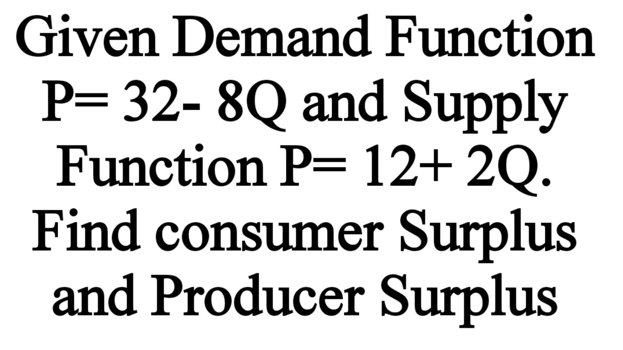
Consumers' Surplus , Producers' Surplus & Total Surplus from demand & supply Functions #PS

Supply and demand in 8 minutes

Price Ceiling Practice Problem | (STEP-BY-STEP SOLUTION)| PART 1 | Think Econ
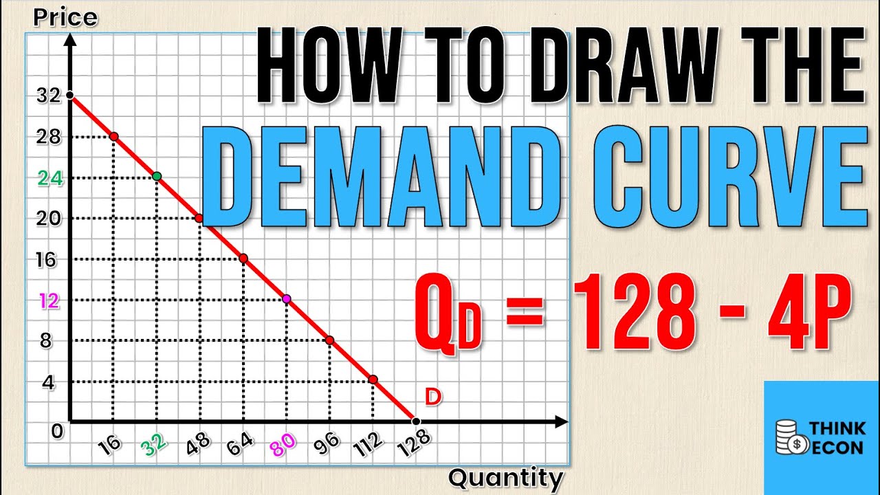
How to Draw the DEMAND CURVE (Using the DEMAND EQUATION) | Think Econ
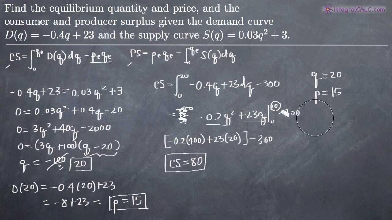
Consumer and Producer Surplus (KristaKingMath)

equilibrium price and tax revenue after the imposition a per unit tax from Demand & Supply function
5.0 / 5 (0 votes)
Thanks for rating: