Mathematically Solving for the Income and Substitution Effect of a Price Change
TLDRThis video script explores the income and substitution effects of a price change on consumer behavior. It uses a utility function to demonstrate graphically and mathematically how a price increase for good X from $5 to $10 impacts consumption. The total effect, substitution effect, and income effect are analyzed, showing a decrease in good X consumption and an increase in good Y, holding utility constant. The script concludes with a table summarizing the effects and their implications on consumer spending decisions.
Takeaways
- 📚 The video discusses the income and substitution effects of a price change using a consumer's utility function.
- 📈 The utility function is defined with both goods X and Y raised to the power of 0.5, representing their respective shares in the utility equation.
- 💰 The initial prices for goods X and Y are given as $5 and $2, respectively, and the consumer's income and prices are taken into account.
- 📊 The graphical analysis begins by maximizing utility with the initial prices, resulting in the consumer buying 2 units of X and 5 units of Y at Point A.
- 🔄 The price of good X increases to $10, leading to a new budget constraint and a new optimal consumption point, Point B.
- 🔍 The total effect of the price change is the movement from Point A to Point B, while the substitution effect is the movement from A to C, holding utility constant.
- 🔢 The mathematical derivation involves taking partial derivatives to find the marginal utilities of goods X and Y and setting them equal to their respective prices.
- ✂️ The substitution effect shows a decrease in the consumption of good X by 0.6 units and an increase in good Y by 2 units due to the price increase.
- 💼 The income effect is calculated by comparing the consumption bundles after the price change and finding the difference in consumption of good X (a decrease of 0.4 units) and good Y (a decrease of 2 units).
- 📉 The price increase results in a normal good behavior for both X and Y, where consumption decreases as the price increases, indicating a negative income effect.
- 📋 The video concludes with a summary table that organizes the optimal consumption bundles, total effects, substitution effects, and income effects for both goods.
Q & A
What is the utility function used in the video?
-The utility function used in the video is U(X, Y) = X^0.5 * Y^0.5, where X and Y are both raised to the power of 0.5.
What are the initial prices of good X and good Y in the video?
-The initial prices are $5 for good X and $2 for good Y.
What is the point of tangency at the initial prices?
-The point of tangency at the initial prices is point A, where the consumer buys 2 units of good X and 5 units of good Y.
What happens to the price of good X in the scenario presented in the video?
-The price of good X increases to $10 in the scenario presented in the video.
How does the budget constraint change with the new price of good X?
-The budget constraint becomes steeper with the new price of good X, leading to a new point of tangency at point B.
What is the total effect of the price change on good X?
-The total effect of the price change on good X is a decrease in consumption from 2 units to 1 unit, while the consumption of good Y remains unchanged at 5 units.
What is the substitution effect of the price change on good X?
-The substitution effect of the price change on good X is a decrease in consumption from 2 units to 1.4 units, while the consumption of good Y increases slightly.
How is the income effect calculated in the video?
-The income effect is calculated by comparing the consumption at the new price (point B) with the consumption at the utility constant level (point C), resulting in a decrease in consumption of good X by 0.4 units and good Y by 2 units.
What utility level was used to find the substitution effect?
-The utility level used to find the substitution effect was U = 3.16, which was the utility at the original consumption bundle of 2 units of good X and 5 units of good Y.
How does the consumer's spending decision change due to the price increase of good X?
-Due to the price increase of good X, the consumer's spending decision changes by cutting back on good X by 0.6 units and consuming more of good Y by 2 units, considering the substitution effect.
What is the conclusion of the income effect for both goods X and Y?
-The conclusion of the income effect is that the consumer would buy less of both goods X and Y, with a decrease of 0.4 units for good X and 2 units for good Y, indicating that both are normal goods.
Outlines
📈 Analyzing Price Change Effects on Consumer Behavior
This paragraph introduces a video on the income and substitution effects of a price change using a consumer's utility function. The utility function is given as a function of two goods, X and Y, both raised to the power of 0.5, with income and prices as variables. The video aims to demonstrate graphically and mathematically what happens when the price of good X increases to $10. It shows the initial maximization of utility with the original prices, leading to the consumption of 2 units of X and 5 units of Y at Point A. Then, it illustrates the new maximization with the increased price of X, resulting in consumption at Point B with 1 unit of X and 5 units of Y. The total effect of the price change is moving from A to B, while the substitution effect is moving from A to C, holding utility constant. The income effect is the remaining movement from C to B. The paragraph concludes with a promise to explain the graphical representation mathematically in the following content.
📉 Calculating the Total, Substitution, and Income Effects
The second paragraph delves into the numerical analysis of the effects of a price change on consumer behavior. It starts by reiterating the graphical results from the initial video segment, which showed a decrease in the consumption of good X from 2 to 1 unit and no change in the consumption of good Y, remaining at 5 units. The substitution effect is calculated by evaluating the utility function at the original consumption bundle, finding that utility equals approximately 3.16. The new consumption bundle, with the price of good X at $10, is then used to find the substitution effect, which shows a decrease of 0.6 units in good X and an increase of 2 units in good Y. The income effect is determined by comparing the new consumption bundle with the one found during the substitution effect analysis, revealing a decrease of 0.4 units in good X and 2 units in good Y. The paragraph concludes with a summary table that organizes the optimal consumption bundles, total effects, substitution effects, and income effects for both goods X and Y, highlighting the consumer's spending decisions in response to the price change.
Mindmap
Keywords
💡Utility Function
💡Price Change
💡Substitution Effect
💡Income Effect
💡Budget Constraint
💡Indifference Curve
💡Marginal Utility
💡Optimal Consumption Bundle
💡Tangency Point
💡Total Effect
Highlights
The video explores the income and substitution effects of a price change using a consumer's utility function.
The utility function is defined with both goods X and Y raised to the power of 0.5.
The initial prices for goods X and Y are $5 and $2, respectively.
The graphical approach is used to maximize utility and find the initial tangency point A.
At point A, the consumer buys 2 units of good X and 5 units of good Y.
The price of good X increases to $10, leading to a new budget constraint and tangency point B.
At point B, consumption shifts to 1 unit of good X and remains at 5 units of good Y.
The total effect of the price change is the movement from A to B.
The substitution effect is represented by the movement from A to C, holding utility constant.
At point C, the consumer would buy 1.4 units of X and 7 units of Y with the new budget constraint.
The income effect is the remaining movement from C to B after accounting for substitution.
Graphical representation helps to understand the mathematical calculations involved.
The marginal utility of good X and the marginal utility of good Y are derived through partial derivatives.
The utility-maximizing condition sets the marginal utility per dollar spent on each good equal to each other.
The consumption bundle at the new price point is found to be 1 unit of X and 5 units of Y.
The substitution effect leads to a decrease in good X consumption by 0.6 units and an increase in good Y consumption by 2 units.
The income effect shows a decrease in consumption of both goods, indicating normal goods behavior.
A summary table is provided to simplify the understanding of the total, substitution, and income effects.
Transcripts
Browse More Related Video
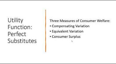
Perfect Substitutes Utility: Compensating Variation, Equivalent Variation, and Consumer Surplus
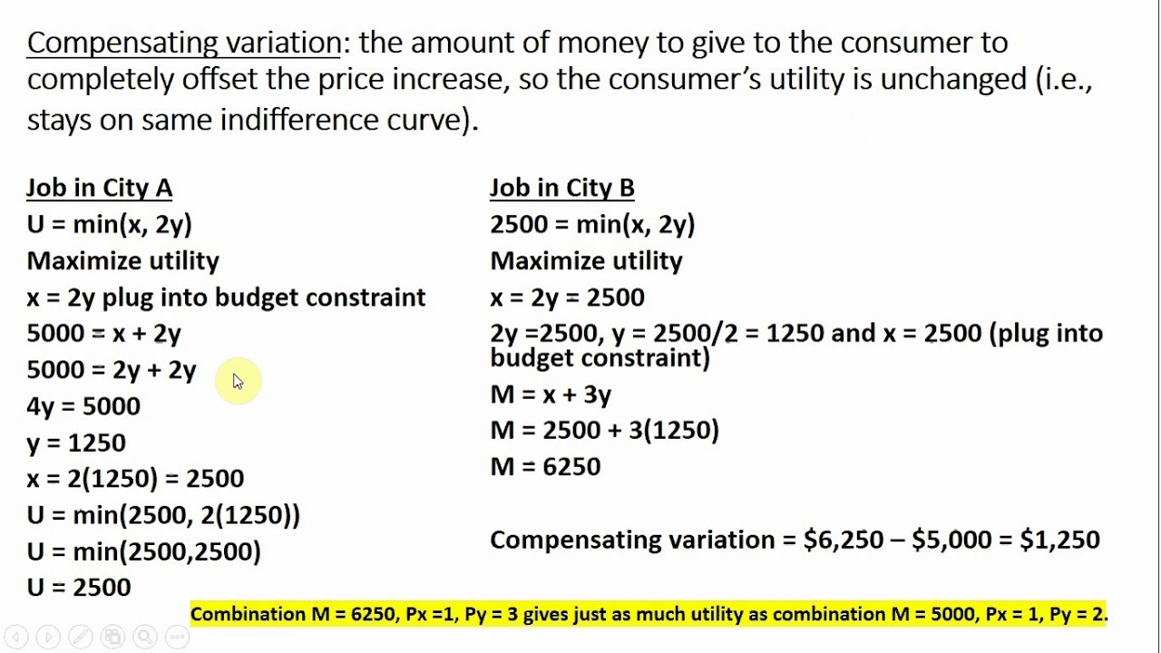
Consumer Welfare: Compensating Variation & Equivalent Variation

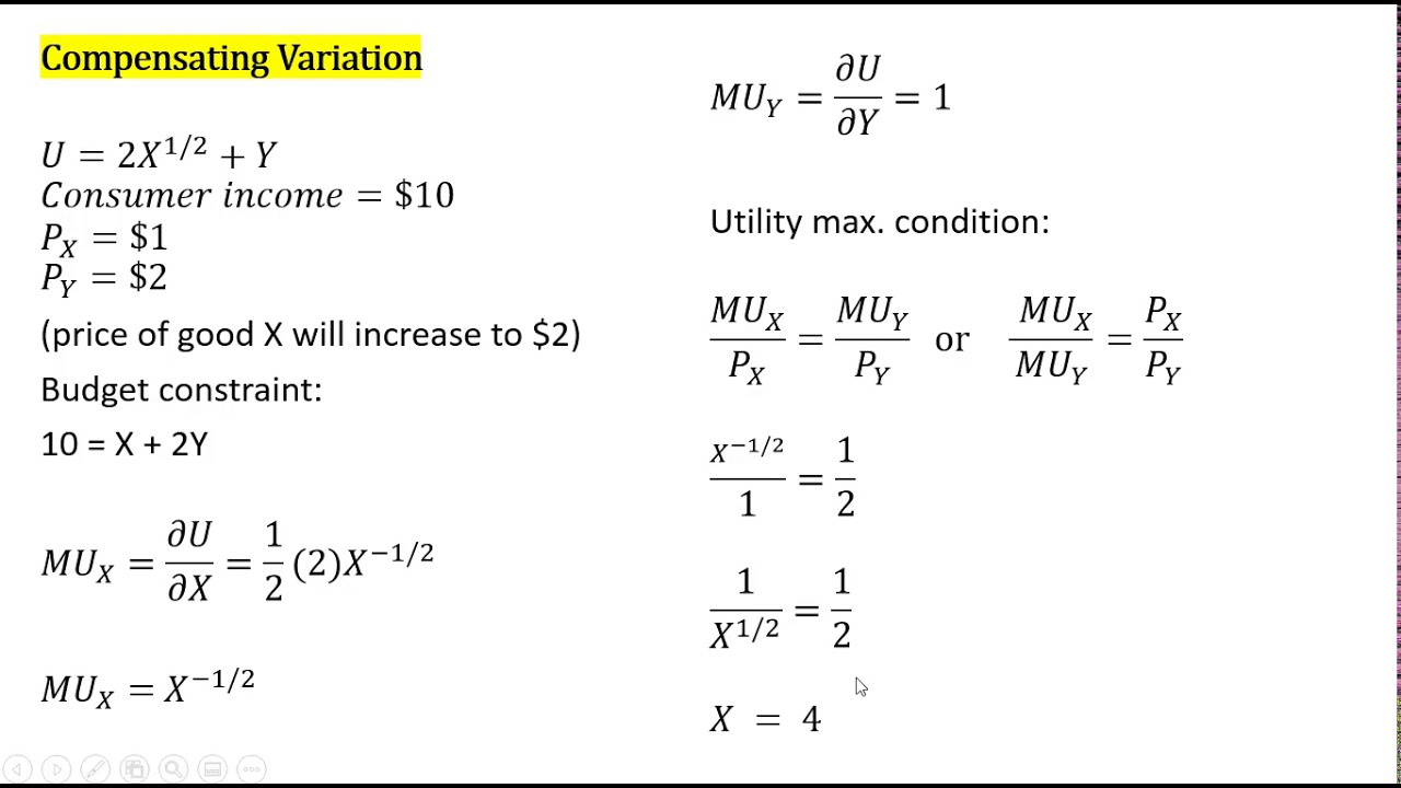
How to Calculate Compensating Variation and Equivalent Variation
Three Measures of Consumer Welfare: Compensating Variation, Equivalent Variation, Consumer Surplus
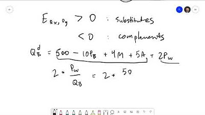
Managerial Economics 2.5: More Elasticity

16. Compensating Variation and Equivalent Variation
5.0 / 5 (0 votes)
Thanks for rating: