How to Calculate Compensating Variation and Equivalent Variation
TLDRThis video explores an alternative method for calculating compensating and equivalent variations resulting from a price change using a consumer's Cobb Douglas utility function. It demonstrates utility maximization under different price scenarios for goods X and Y, with varying incomes and prices. The script calculates compensating variation as the amount the consumer would forego to maintain pre-price change utility, and equivalent variation as the income adjustment needed to achieve the same post-price change utility, verifying both through utility maximization under altered constraints.
Takeaways
- 📚 The video introduces an alternative method to calculate compensating and equivalent variations resulting from a price change.
- 📈 A consumer's Cobb-Douglas utility function is used with specific utility values for goods X and Y.
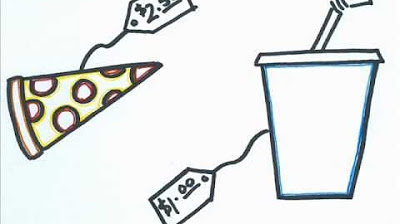
- 💰 The consumer has a fixed income of 80 dollars and faces initial prices of 4 dollars per unit for good X and 1 dollar per unit for good Y.
- 🧩 The initial budget constraint is established as 80 = 4X + Y, leading to the determination of the utility-maximizing quantities of goods X and Y.
- ⚖️ The marginal rate of substitution (MRS) is equated to the ratio of the prices of the goods to find the optimal consumption bundle.
- 🔍 After finding the initial consumption levels (X=10, Y=40), the price of good X decreases from 4 to 2 dollars, prompting a recalculation of the optimal consumption.
- 📉 The new budget constraint is set up with the reduced price for good X, leading to new optimal quantities (X=20, Y=40).
- 🔄 The utility level post-price change is calculated to be 800, indicating an increase in consumer satisfaction.
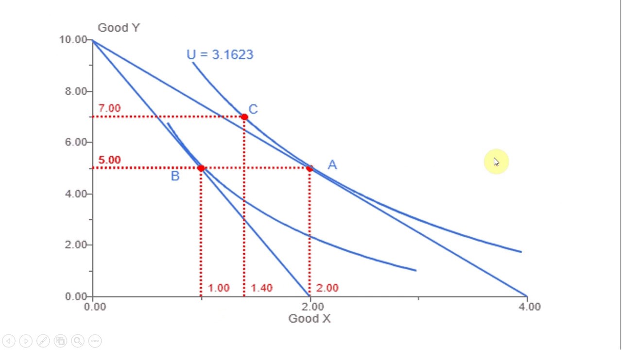
- 🔄 The concept of compensated demand is introduced to find the quantity of good X that would maintain the initial utility level after the price change.
- 💡 Compensating variation is calculated as the integral of the compensated demand between the old and new prices of good X, resulting in a value of 23.43 dollars.
- 💸 The equivalent variation is determined by integrating the compensated demand at the new utility level, yielding a value of 33.137 dollars.
- 🔍 The video concludes with a verification step, confirming that the compensating and equivalent variations accurately reflect the utility levels before and after the price change.
Q & A
What is the Cobb Douglas utility function mentioned in the video?
-The Cobb Douglas utility function is a specific type of utility function used in economics that assumes the utility of a consumer is a product of the quantities of different goods raised to some constant power. In the video, the utility function is given by U = X * Y, where X and Y are the quantities of two goods.
What is the consumer's income and the initial prices of goods X and Y in the video?
-The consumer has an income of 80 dollars. The initial price of good X is 4 dollars per unit, and the price of good Y is 1 dollar per unit.
How is the budget constraint derived in the video?
-The budget constraint is derived by setting the total income equal to the sum of the products of the quantities of each good and their respective prices. In this case, it is 80 = 4X + Y.
What is the marginal rate of substitution (MRS) and how is it used in the video?
-The marginal rate of substitution (MRS) is the rate at which a consumer is willing to trade one good for another while maintaining the same level of utility. In the video, the MRS is set equal to the ratio of the prices of the two goods to find the utility maximizing outcome.
What is the utility maximizing quantity of goods X and Y before the price change of good X?
-Before the price change, the utility maximizing quantities are X = 10 units and Y = 40 units, which are found by solving the budget constraint and the MRS condition.
What happens to the price of good X and what is the new budget constraint?
-The price of good X falls from 4 dollars to 2 dollars per unit. The new budget constraint becomes 80 = 2X + Y.
How is the new utility maximizing quantity of goods X and Y calculated after the price change of good X?
-After the price change, the MRS is recalculated as the ratio of the new prices, leading to Y = 2X. Solving this with the new budget constraint gives X = 20 units and Y = 40 units.
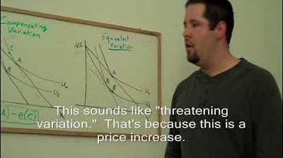
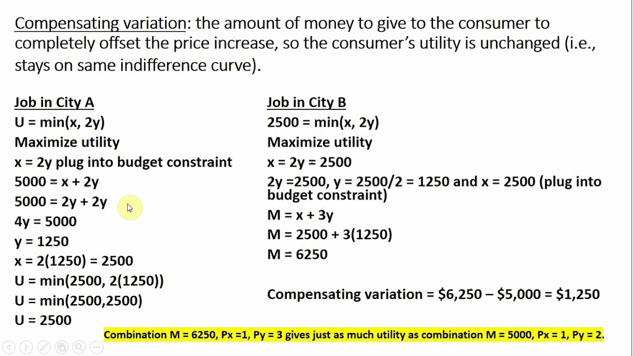
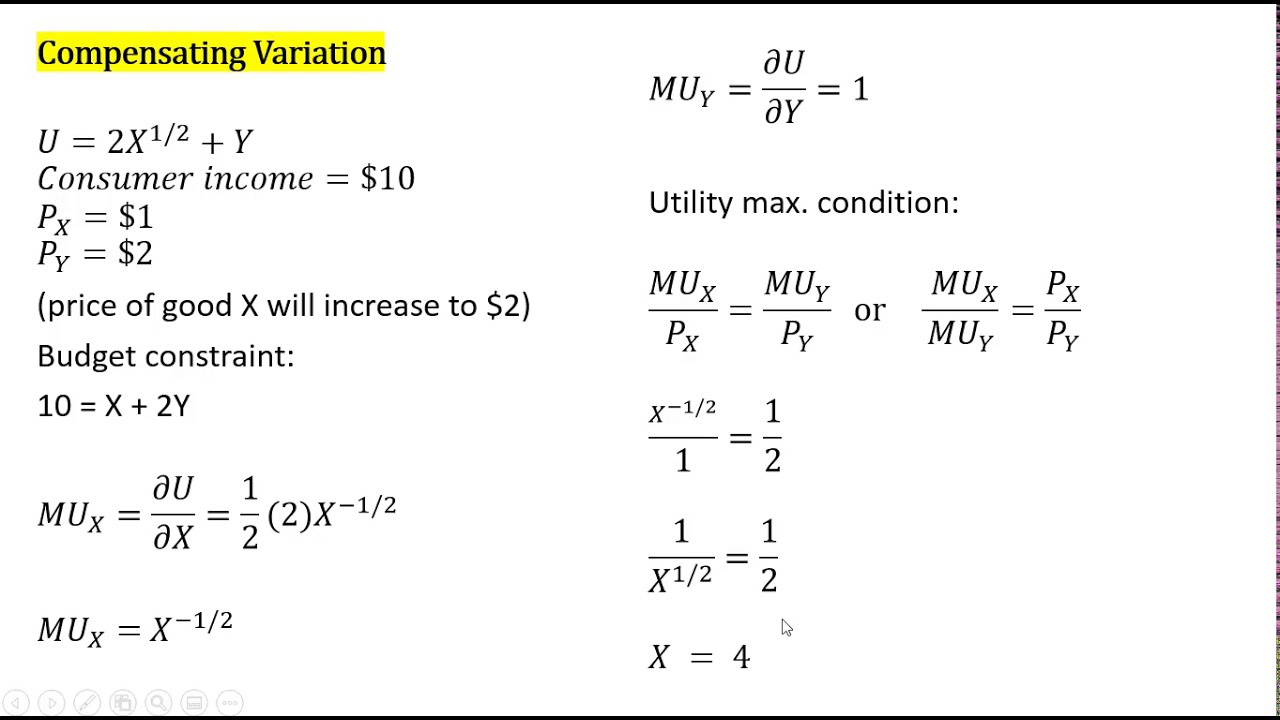
What is compensating variation and how is it calculated in the video?
-Compensating variation measures the amount of money the consumer is willing to give up after a price decrease to have the same level of utility as before the price decrease. In the video, it is calculated by integrating the compensated demand for good X between the old and new prices of good X.
What is the result of the compensating variation calculation in the video?
-The compensating variation is calculated to be 23.43 dollars, which means the consumer would be willing to give up this amount of money to maintain the same utility level after the price decrease.
What is equivalent variation and how is it calculated in the video?
-Equivalent variation measures the amount of money the consumer must receive at original prices to have the same level of utility after a price decrease. In the video, it is calculated by integrating the compensated demand for good X evaluated at the utility after the price change between the old and new prices of good X.
What is the result of the equivalent variation calculation in the video?
-The equivalent variation is calculated to be 33.137 dollars, which means the consumer would need to receive this amount of money before the price decrease to achieve the same utility level as after the price decrease with the original income.
Outlines
📚 Calculating Compensating and Equivalent Variations
This paragraph introduces the concept of calculating compensating and equivalent variations from a price change using a consumer's Cobb Douglas utility function. The scenario involves a consumer with a fixed income and two goods with given prices. The utility function is set with specific marginal utilities for goods X and Y. The initial budget constraint and utility maximizing outcome are established, leading to the consumer's optimal consumption quantities. Following a price decrease for good X, the paragraph explores the re-optimization process and introduces the concepts of compensating variation and equivalent variation, which measure the impact of the price change on consumer welfare.
🔍 Detailed Analysis of Compensating and Equivalent Variations
The second paragraph delves deeper into the calculations of compensating and equivalent variations. It starts by re-establishing the utility maximizing condition with the new price for good X and deriving the new consumption quantities. The paragraph then explains how to find the compensated demand for good X by manipulating the utility function and the price ratio. The compensating variation is calculated as the integral of the compensated demand between the old and new prices of good X, resulting in a specific monetary value that represents the income change needed to maintain the same utility level after the price decrease. The paragraph also verifies this result by showing the new consumption quantities and utility level after reducing the consumer's income by the compensating variation amount. Finally, it calculates the equivalent variation, which is the amount that, if given to the consumer before the price change, would result in the same utility level as after the price change with the original income. The paragraph concludes with a verification of the equivalent variation result.
Mindmap
Keywords
💡Cobb Douglas Utility Function
💡Marginal Rate of Substitution (MRS)
💡Budget Constraint
💡Compensating Variation
💡Equivalent Variation
💡Price Change
💡Income Effect
💡Utility Maximization
💡Compensated Demand
💡Integral
💡Price Ratio
Highlights
Introduction to an alternative approach for calculating compensating and equivalent variation from a price change.
Presentation of a consumer's Cobb Douglas utility function with specific utility for goods X and Y.
Given consumer income and prices of goods X and Y, establishing the initial budget constraint.
Utility maximizing outcome by setting the marginal rate of substitution equal to the price ratio.
Solving for the quantity of good Y in terms of good X using the utility function.
Substituting the derived relationship into the budget constraint to find the optimal quantities of goods X and Y.
Calculation of the initial level of utility with the given quantities of goods X and Y.
Scenario of a price decrease for good X and the intention to calculate compensating and equivalent variations.
Re-establishing the budget constraint with the new price for good X.
Deriving the new demand for good Y in terms of good X with the updated price ratio.
Solving for the new quantities of goods X and Y after the price change for good X.
Calculation of the new level of utility with the updated quantities and prices.
Introduction to the concept of compensated demand for good X.
Derivation of the compensated demand for good X using utility maximizing conditions.
Calculation of compensating variation by integrating compensated demand over the price change.
Verification of compensating variation through a utility maximization problem with reduced income.
Introduction to the equivalent variation and its calculation method.
Calculation of equivalent variation by integrating compensated demand at new utility levels and prices.
Verification of equivalent variation through a utility maximization problem with additional income at original prices.
Conclusion summarizing the compensating and equivalent variations and their implications for consumer utility.
Transcripts
Browse More Related Video
16. Compensating Variation and Equivalent Variation
Consumer Welfare: Compensating Variation & Equivalent Variation
Perfect Substitutes Utility: Compensating Variation, Equivalent Variation, and Consumer Surplus
Three Measures of Consumer Welfare: Compensating Variation, Equivalent Variation, Consumer Surplus
Episode 18: Consumer Equilibrium
Mathematically Solving for the Income and Substitution Effect of a Price Change
5.0 / 5 (0 votes)
Thanks for rating: