Live Day 2- Basic To Intermediate Statistics
TLDRIn this educational live session, the instructor engages with the audience on statistics fundamentals, particularly for data science. The session covers measures of central tendency, including mean, median, and mode, and their resilience to outliers. It progresses to measures of dispersion, such as variance and standard deviation, explaining their importance in data spread analysis. The instructor also introduces concepts like percentiles, quartiles, and the interquartile range, demonstrating how to identify and handle outliers using box plots. The session is interactive, with the instructor seeking audience confirmation and corrections throughout, and promoting a comprehensive learning platform offering a wide range of courses.
Takeaways
- 🎙️ The speaker begins by ensuring their audio is audible and requests engagement through likes, setting a casual and interactive tone for the session.
- 📚 The session includes a review of basic statistical concepts and progresses to intermediate topics, specifically for data science applications.
- 📈 The speaker introduces measures of central tendency, including arithmetic mean, median, and mode, explaining their relevance and calculation methods.
- 🔢 An arithmetic mean formula is provided for both population (μ) and sample (x̄), highlighting the importance of understanding the formulas and notation used in statistics.
- 📉 The impact of outliers on statistical measures like mean is discussed, emphasizing the need for caution when dealing with extreme values in a dataset.
- 📊 The concept of central tendency is explained as a method to find the center of a data distribution, with mean, median, and mode serving different purposes based on data characteristics.
- 📚 The speaker provides a detailed example of calculating the mean and discusses the process of finding the median in both odd and even numbered datasets.
- 🤔 The session touches on the importance of understanding data distribution through visualization techniques like histograms and PDFs, which will be further elaborated in future lessons.
- 📈 The speaker moves on to discuss measures of dispersion, including variance and standard deviation, explaining their significance in understanding data spread.
- 🧩 The concept of percentiles and quartiles is introduced as a method to identify outliers and understand the distribution of data within certain intervals.
- 📊 The 'five number summary' is explained as a tool for data analysis, which includes minimum, first quartile (Q1), median, third quartile (Q3), and maximum, and is used to create box plots for visualizing data distribution and outliers.
Q & A
What is the purpose of a box plot in data analysis?
-A box plot is used to determine the distribution of data, identify outliers, and visualize the spread and skewness of the data. It shows the minimum, first quartile (Q1), median, third quartile (Q3), and maximum values.
How do you calculate the interquartile range (IQR)?
-The interquartile range (IQR) is calculated as the difference between the third quartile (Q3) and the first quartile (Q1). The formula is IQR = Q3 - Q1.
What is the difference between population variance and sample variance?
-Population variance is calculated using the formula: σ² = Σ (Xi - μ)² / N, where N is the population size. Sample variance uses the formula: s² = Σ (Xi - X̄)² / (n - 1), where n is the sample size. The sample variance divides by (n - 1) to correct for bias in the estimation of the population variance.
Why is the sample variance formula divided by (n-1) instead of n?
-The sample variance formula is divided by (n-1) to account for the degrees of freedom in the sample and to provide an unbiased estimate of the population variance. This correction is known as Bessel's correction.
How do you calculate the median from a dataset?
-To calculate the median, sort the dataset and find the middle value. If the number of observations is odd, the median is the middle value. If the number of observations is even, the median is the average of the two middle values.
What is a percentile and how is it used?
-A percentile is a value below which a certain percentage of observations in a dataset fall. For example, the 25th percentile (Q1) is the value below which 25% of the data lies. Percentiles are used to understand the relative standing of a value within a dataset.
How do you determine the percentile rank of a specific value in a dataset?
-To determine the percentile rank of a specific value, use the formula: Percentile Rank = (Number of values below X / Total number of values) * 100. This formula calculates the percentage of values that are less than the given value X.
What is the role of central tendency in statistics?
-Central tendency refers to measures used to determine the center of a distribution of data. The main measures of central tendency are the mean, median, and mode, which provide insights into the average, middle, and most frequent values in the dataset, respectively.
How do you calculate the standard deviation from variance?
-The standard deviation is the square root of the variance. For a population, it is calculated as σ = √σ², and for a sample, it is calculated as s = √s². Standard deviation provides a measure of the average distance of each data point from the mean.
Why is it important to remove outliers from a dataset?
-Outliers can significantly affect the results of data analysis by skewing the mean and other statistical measures, leading to inaccurate conclusions. Removing outliers ensures a more accurate representation of the data's central tendency and dispersion.
Outlines
🔊 Session Introduction and Community Enrollment
The speaker begins by checking if the audience can hear them and encourages likes on their platform. They remind participants to join a community session where materials from the previous day's video are available. The speaker emphasizes the importance of enrolling in the community session for access to live streams and materials. They confirm that everyone is enrolled and prepare to start the session, transitioning to an intermediate data science topic discussion. The speaker also addresses the issue of background visibility and adjusts it based on audience feedback.
📚 Review of Previous Day's Statistics Session
The speaker reviews the topics covered in the previous session, focusing on statistics. They ask attendees to recall the topics discussed, specifically mentioning arithmetic mean for both population and sample. The speaker corrects a mistake made during the calculation of the mean and emphasizes the importance of understanding the formulas and concepts. They also note that the PDF materials have been updated and are available in the resource folder of the specific video.
📈 Understanding Central Tendency Measures
The speaker explains the concept of central tendency, which includes mean, median, and mode. They discuss the arithmetic mean for both population and sample, highlighting the importance of notation in the industry. The speaker then introduces the median as a measure that is less affected by outliers, demonstrating this with an example that includes an outlier. They compare the impact of outliers on mean and median and explain why median is preferred in such cases.
📊 Impact of Outliers on Data Distribution
The speaker delves into the impact of outliers on data distribution, using the median as an example. They illustrate how adding an outlier can significantly affect the mean but has a lesser impact on the median. The speaker emphasizes the importance of being cautious with outliers in data science and statistics and mentions that techniques to handle outliers will be discussed later, including percentiles.
🔢 Exploring Mode and Handling Missing Data
The speaker discusses the mode as a measure of central tendency, explaining how it is the most frequent element in a data set. They provide examples of how mode can be used with categorical variables and how it can be particularly useful for handling missing data by replacing missing values with the most frequent occurring element in the data set.
📉 Measures of Dispersion: Variance and Standard Deviation
The speaker introduces measures of dispersion, specifically variance and standard deviation. They explain that dispersion refers to the spread of data and differentiate it from measures of central tendency. The speaker defines population variance and sample variance, highlighting the use of 'n-1' in sample variance calculations. They also discuss the importance of understanding these concepts for interviews and real-world applications.
📝 Calculation and Interpretation of Variance
The speaker provides a step-by-step calculation of variance using a data set and explains the process of squaring differences from the mean. They emphasize the importance of squaring these differences as per the variance formula. The speaker then interprets the calculated variance, explaining that a higher variance indicates a greater spread of data.
📊 Understanding Standard Deviation and Data Spread
The speaker explains standard deviation as the square root of variance and discusses its relationship with data spread. They use a graphical representation to illustrate how a smaller standard deviation indicates a more concentrated data distribution, while a larger standard deviation indicates a more dispersed distribution. The speaker also explains how standard deviation can be used to determine the range of data within one standard deviation of the mean.
🗄️ Introduction to Percentiles and Quartiles
The speaker introduces the concept of percentiles and quartiles as a method to find outliers and understand data distribution. They explain the definition of a percentile and provide a real-life example from a YouTube ranking. The speaker emphasizes the importance of understanding percentiles for various exams and real-world applications.
🔢 Calculating Percentile Ranks and Understanding Their Meaning
The speaker demonstrates how to calculate percentile ranks with a data set and explains the meaning behind the values obtained. They clarify that a percentile rank indicates the percentage of observations below a certain value in a distribution. The speaker also provides an example to find the percentile ranking of a specific value and gives an assignment to the audience to calculate another percentile rank.
📈 Determining Percentile Values and Revisiting Dispersion
The speaker guides the audience through determining the value at a specific percentile ranking, using a formula that involves the position in the data set. They discuss the concept of dispersion again, emphasizing its importance in understanding the spread of data. The speaker also addresses a technical issue with the background during the session, showing their adaptability to unexpected changes.
📊 Calculating the Five-Number Summary and Identifying Outliers
The speaker explains the concept of the five-number summary, which includes minimum, first quartile (Q1), median, third quartile (Q3), and maximum. They demonstrate how to calculate these values and use them to identify and remove outliers from a data set. The speaker introduces the lower and upper fences, which are used in conjunction with the interquartile range (IQR) to determine outliers.
📈 Computing the Interquartile Range (IQR) and Adjusting for Outliers
The speaker continues the discussion on removing outliers by computing the interquartile range (IQR) and adjusting the lower and higher fences. They provide a clear explanation of how to calculate the IQR and use it to define the fences. The speaker then identifies the outlier in the provided data set and explains the process of adjusting the data set by removing the outlier.
📊 Constructing a Box Plot and Understanding Its Components
The speaker describes how to construct a box plot using the five-number summary and explains the significance of each component of the box plot. They illustrate the process of drawing a box plot and explain how it can be used for data visualization and outlier detection. The speaker also discusses the importance of understanding box plots for data science applications.
📚 Wrapping Up the Session and Previewing Future Topics
The speaker concludes the session by summarizing the topics covered and providing a preview of what will be discussed in future sessions. They mention the intention to cover various distributions, confidence intervals, p-values, hypothesis testing, and more advanced statistical concepts. The speaker also encourages the audience to share the session with friends and subscribe to the channel for updates on future content.
🎓 Promoting One Neuron Platform and Its Comprehensive Course Offerings
The speaker promotes the One Neuron platform, highlighting its extensive course offerings across various domains such as data science, machine learning, AI/ML, and more. They mention the platform's lifetime subscription model and the opportunity for users to request new courses or modules. The speaker also provides a discount code for the platform and encourages the audience to take advantage of the available courses.
📅 Final Session Reminder and Encouragement for Continued Learning
The speaker reminds the audience of the next session's timing and encourages them to subscribe and like the video for updates. They express gratitude for the audience's participation and reiterate the importance of continuing education and learning. The speaker also mentions the inclusion of courses like linear algebra, GCP, AWS, and others on the One Neuron platform, emphasizing the platform's comprehensive nature.
Mindmap
Keywords
💡Central Tendency
💡Mean
💡Median
💡Mode
💡Dispersion
💡Variance
💡Standard Deviation
💡Outliers
💡Percentile
💡Box Plot
Highlights
Introduction to the session with an emphasis on community involvement and the availability of materials.
Transition from basic to intermediate statistics for data science, outlining the day's topics.
Explanation of the measure of central tendency, including mean, median, and mode.
Discussion on the impact of outliers on statistical measures like the mean.
Introduction to the concept of median as a more robust measure against outliers.
Explanation of mode as a measure of central tendency, especially useful for categorical data.
Introduction to measure of dispersion, including variance and standard deviation.
Clarification on the difference between population variance and sample variance.
Illustration of how to calculate variance and standard deviation with an example dataset.
Importance of understanding dispersion in data through variance and standard deviation.
Introduction to percentiles and quartiles as a method to identify outliers.
Explanation of how to calculate percentiles and their significance in data analysis.
Demonstration of how to find the value at a specific percentile rank.
Introduction to the five-number summary and its role in data description.
Technique to remove outliers using the interquartile range (IQR) and fences.
Application of box plots in data visualization and outlier detection.
Discussion on the use of the lower and upper fences for identifying outliers.
Promotion of the One Neuron platform offering a wide range of courses for a lifetime subscription.
Transcripts
Browse More Related Video
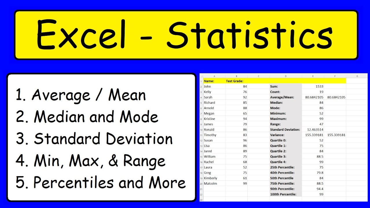
Statistics - Excel
Elementary Statistics - Chapter 3 Describing Exploring Comparing Data Measure of Central Tendency
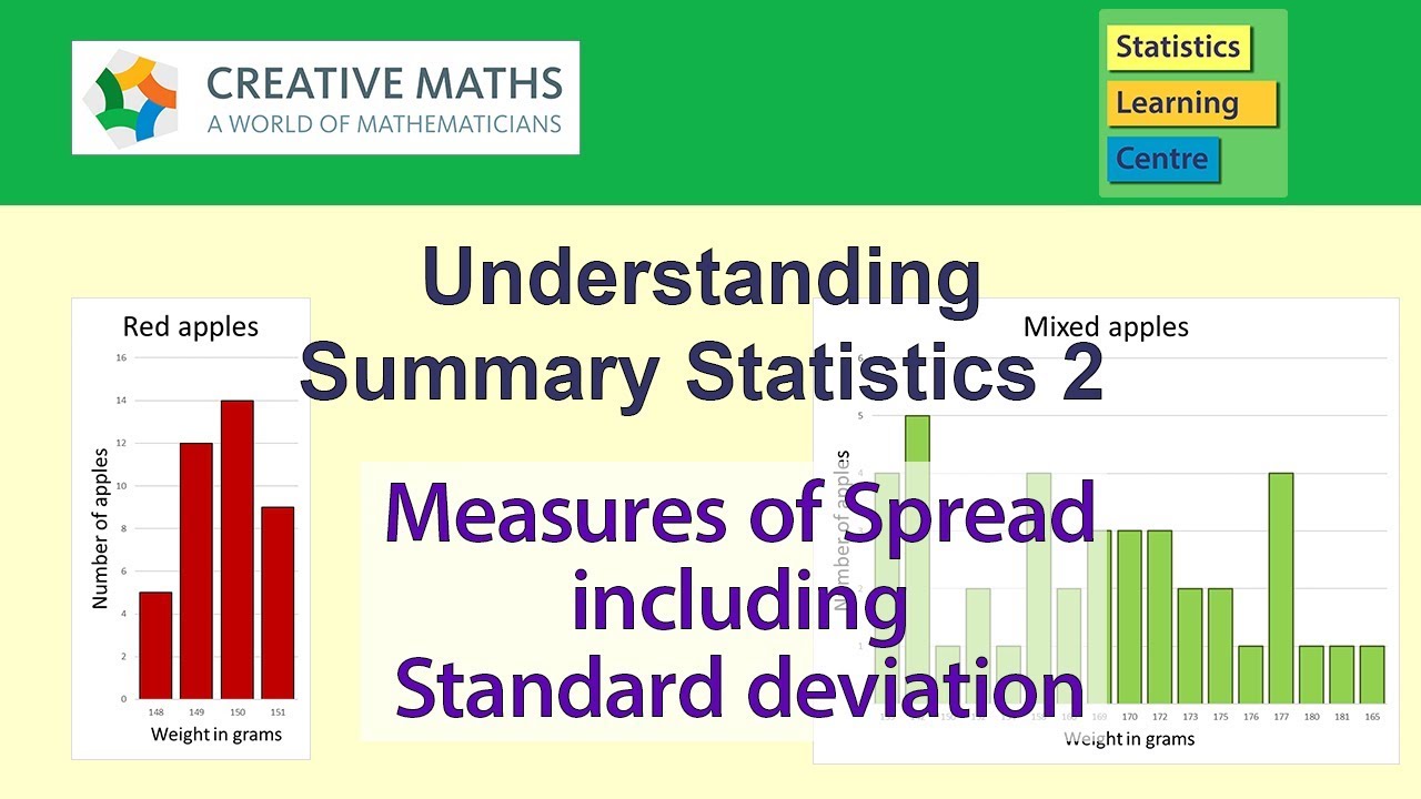
Understanding Standard deviation and other measures of spread in statistics
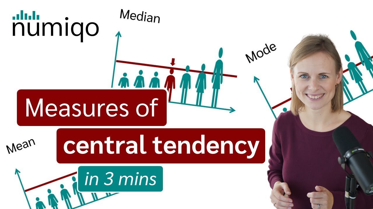
Mean, Median and Mode - Measures of Central Tendency

What is Descriptive Statistics? A Beginner's Guide to Descriptive Statistics!

Elementary Stats Lesson #3 A
5.0 / 5 (0 votes)
Thanks for rating: