Differential Equations with Velocity and Acceleration (Differential Equations 7)

Professor Leonard

28 Sept 201843:59

EducationalLearning

32 Likes 10 Comments

TLDRThis video script delves into the concept of second-order differential equations, focusing on their application in modeling real-world scenarios such as motion, where position, velocity, and acceleration are interconnected. The lesson explains how to solve these equations through a step-by-step process of integration, emphasizing the importance of initial conditions in finding particular solutions. The examples provided illustrate how to translate theoretical concepts into practical problem-solving, highlighting the relevance of differential equations in understanding and predicting the behavior of various physical systems.

Takeaways

📚 The lesson focuses on solving second-order differential equations by integrating twice to find the function y, given a second derivative of y equals a function of X.
🌐 In second-order differential equations, each integration introduces an arbitrary constant, resulting in two constants for second-order equations.
🔄 The process involves converting the second derivative to a first derivative through integration, and then from the first derivative to the original function (position) with another integration.
💡 The key to solving these equations is understanding the relationship between position, velocity, and acceleration: the derivative of position is velocity, and the second derivative is acceleration.
📈 To find a particular solution, two initial conditions are needed: one for the initial position and one for the initial velocity.
🌟 The script provides examples of how to apply this process to various scenarios, including those with non-constant acceleration functions.
🧩 The examples demonstrate the importance of integrating acceleration to find velocity, and then integrating velocity to find the position function.
🔧 The script emphasizes the practical application of these concepts, such as modeling the motion of objects in terms of their acceleration, velocity, and position over time.
📊 The process is illustrated with examples that include integrating more complex functions, like those involving square roots and trigonometric functions.
🎯 The script encourages viewers to practice solving these problems to reinforce understanding and prepare for more complex applications in future lessons.
🚀 The next video will focus on real-world examples involving cars skidding and jumping on planes with different gravity, providing a more tangible application of the concepts learned.

Q & A

What is the main topic of the video?
-The main topic of the video is solving second-order differential equations, specifically those related to acceleration, velocity, and position.
How does the video introduce the concept of second-order differential equations?
-The video introduces the concept by discussing the basic idea of differential equations and then extending it to second-order differential equations, emphasizing the relationship between the derivatives and physical quantities like acceleration, velocity, and position.
What is the method used in the video to solve second-order differential equations?
-The method used is integration. The video explains that by integrating the equation twice, one can obtain the function for the variable of interest (e.g., position from acceleration).
Why are two arbitrary constants introduced when solving second-order differential equations?
-Two arbitrary constants are introduced because each integration adds an undetermined constant. These constants represent the initial conditions that need to be determined to find a particular solution.
How does the video relate the derivatives to physical quantities?
-The video relates the first derivative to velocity (as the rate of change of position) and the second derivative to acceleration (as the rate of change of velocity), demonstrating how these mathematical concepts apply to real-world physical systems.
What are the initial conditions needed to solve a second-order differential equation?
-To solve a second-order differential equation, one needs two initial conditions: an initial position and an initial velocity. These are necessary to determine the two arbitrary constants introduced by the two integrations.
How does the video handle non-constant acceleration in the examples?
-For non-constant acceleration, the video demonstrates the process of integrating the acceleration function twice, using initial conditions to solve for the arbitrary constants, and obtaining the functions for velocity and position.
What is the significance of the initial conditions in the context of the video?
-Initial conditions are crucial because they allow us to find the particular solution to the differential equation. They provide the necessary information about the state of the system at the starting point in time.
What is the role of integration in solving these types of differential equations?
-Integration is used to reverse the process of differentiation, effectively 'undoing' the second derivative to find the first derivative (velocity), and then the original function (position). It's a key step in transforming the differential equation into a solvable form.
How does the video prepare the viewer for future content?
-The video sets the stage for future content by mentioning that upcoming videos will include more complex examples and real-world applications, such as cars skidding and jumping on planes with different gravity, to further solidify the understanding of differential equations.

Outlines

00:00

📚 Introduction to Second-Order Differential Equations

This paragraph introduces the concept of second-order differential equations, focusing on the idea of extending the basic understanding of first-order differential equations. It explains how to solve second-order equations through integration, using the example of a function's second derivative being equal to a function of X. The key concept highlighted is the relationship between acceleration, velocity, and position, and how these can be modeled using differential equations.

05:02

🌟 Integration Process and Arbitrary Constants

The paragraph delves into the process of integrating second-order differential equations, emphasizing the role of arbitrary constants. It explains that integrating twice is required to solve for the function y, and that each integration introduces a new arbitrary constant. The importance of initial conditions, such as initial position and velocity, is discussed in the context of finding particular solutions to these equations.

10:03

🚀 Applying Differential Equations to Motion

This section applies the concepts of differential equations to the real-world scenario of motion, specifically acceleration, velocity, and position. It explains how the derivative of position gives velocity, and the second derivative gives acceleration. The paragraph outlines the process of integrating acceleration to find velocity and then integrating velocity to find position, while also highlighting the need for initial conditions to solve for specific values.

15:03

🧩 Solving with Constant Acceleration

The paragraph focuses on solving second-order differential equations when acceleration is constant. It simplifies the process by showing how to integrate the acceleration function to find the velocity function and then another integration to find the position function. The importance of initial velocity and position in determining the particular solution is reiterated, with a clear example provided to illustrate the process.

20:05

🔄 Examples with Non-Constant Acceleration

This section presents examples of solving second-order differential equations with non-constant acceleration. It explains that while the basic process of integration remains the same, the presence of non-constant functions requires a more nuanced approach. The paragraph emphasizes the need for initial conditions and provides a step-by-step guide to solving the equations, including the use of substitution and dealing with arbitrary constants.

25:05

🎯 Finalizing the Solution with Initial Conditions

The paragraph concludes the discussion on solving second-order differential equations by showing how to finalize the solution using initial conditions. It reiterates the process of integrating acceleration to find velocity and then integrating velocity to find position, while also highlighting the importance of initial conditions in determining the specific values of the arbitrary constants. The paragraph ends with a summary of the key concepts and an encouragement for viewers to practice solving these types of problems.

Mindmap

Keywords

💡Differential Equations

Differential Equations are mathematical equations that involve an unknown function and its derivatives. In the context of the video, they are used to model real-world situations such as motion, where the equations relate variables like acceleration, velocity, and position. The video focuses on second-order differential equations, which involve the second derivative of a function.

💡Integration

Integration is a mathematical process that is the reverse of differentiation. It involves finding a function whose derivative is a given function. In the video, integration is used to solve differential equations by transforming them into a form that can be analyzed with initial conditions, allowing the determination of functions like velocity and position from acceleration.

💡Second Derivative

The second derivative of a function is the derivative of the first derivative. It measures the rate of change of the rate of change of the function's value. In physics, the second derivative of position with respect to time represents acceleration, making it a key concept in modeling motion.

💡Antiderivative

An antiderivative, also known as an indefinite integral, is a function whose derivative is a given function. In the context of differential equations, finding the antiderivative is a crucial step in solving the equation, as it helps to determine the function that satisfies the equation's conditions.

💡Arbitrary Constants

Arbitrary constants are values that are added to the antiderivative when integrating a function. They represent the uncertainty in the initial conditions of the function being integrated. In differential equations, each integration adds an arbitrary constant, which must be determined by initial conditions or boundary values.

💡Initial Conditions

Initial conditions are specific values assigned to a function at the starting point of a problem. They are essential for solving differential equations because they allow the determination of the arbitrary constants that arise from integration. In the context of motion, initial conditions might include the initial position and initial velocity of an object.

💡Velocity

Velocity is a measure of the rate of change of position with respect to time. It is the first derivative of position, and in the context of the video, it is used to model how an object's position changes over time when subjected to forces like acceleration.

💡Acceleration

Acceleration is the rate of change of velocity with respect to time. It is the second derivative of position and represents how quickly the velocity of an object is changing. In physics and engineering, acceleration is crucial for understanding motion and the dynamics of objects.

💡Position

Position refers to the location of an object in space. In the context of the video, it is the function from which velocity and acceleration are derived. The position function is found by integrating the velocity function, which itself is found by integrating the acceleration function.

💡Initial Value Problems

Initial value problems are a type of differential equation where the solution is sought based on specified initial conditions. These problems provide a starting point for the unknown function and its derivative, allowing for the determination of the unique solution to the differential equation.

Highlights

Introduction to second-order differential equations and their solutions through integration.

Explaining the relationship between position, velocity, and acceleration in differential equations.

Deriving the position function from a second derivative involving acceleration and velocity.

Discussing the necessity of two arbitrary constants in second-order differential equations and their relation to initial conditions.

Integrating a function with respect to time to find velocity and position functions.

Using initial conditions such as initial position and velocity to solve for the arbitrary constants in the general solution.

Working through examples of acceleration, velocity, and position functions to demonstrate the application of integration in solving differential equations.

Explaining how to handle non-constant acceleration functions in differential equations through integration.

Providing a detailed walkthrough of solving a second-order differential equation with variable coefficients.

Emphasizing the importance of understanding integration and initial conditions for solving practical problems modeled by differential equations.

Demonstrating the process of integrating acceleration to find the velocity function, and then integrating velocity to find the position function.

Highlighting the use of substitution in integration to simplify complex functions and solve differential equations.

Discussing the application of differential equations in real-world scenarios such as modeling the motion of a water balloon thrown from a building.

Outlining the steps to solve a second-order differential equation with non-constant coefficients and multiple integrations.

Providing a comprehensive summary of the process for solving second-order differential equations, including the role of initial conditions and integration.

Encouraging practice and reinforcement of the concepts learned through solving additional examples on one's own.

Transcripts

Browse More Related Video

Calculus AB Homework 7.1 Differential Equations

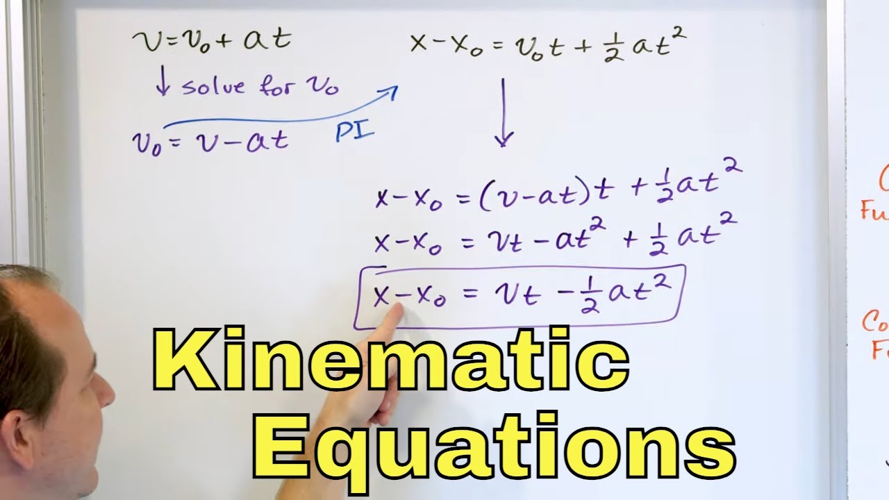
Deriving the Kinematic Equations of Motion w/ Constant Acceleration in Physics - [1-2-13]

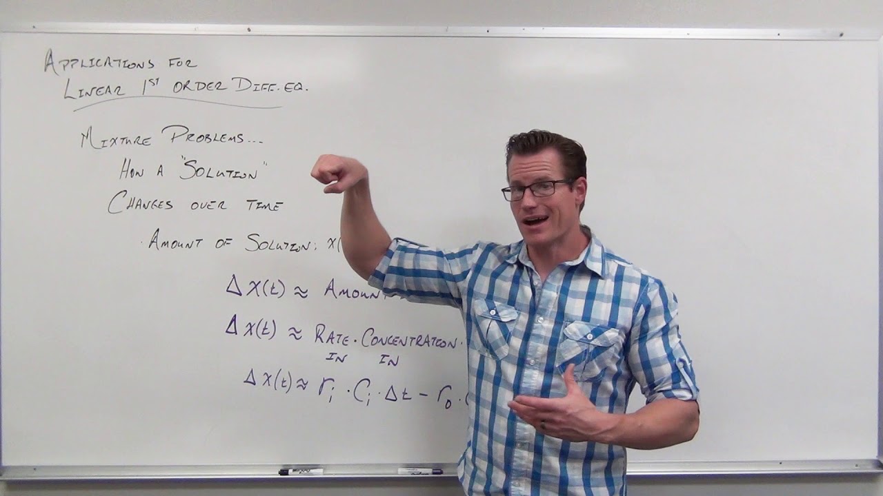
Mixture Problems in Linear Differential Equations (Differential Equations 19)

What is a DIFFERENTIAL EQUATION?? **Intro to my full ODE course**

Simple Differential Equations

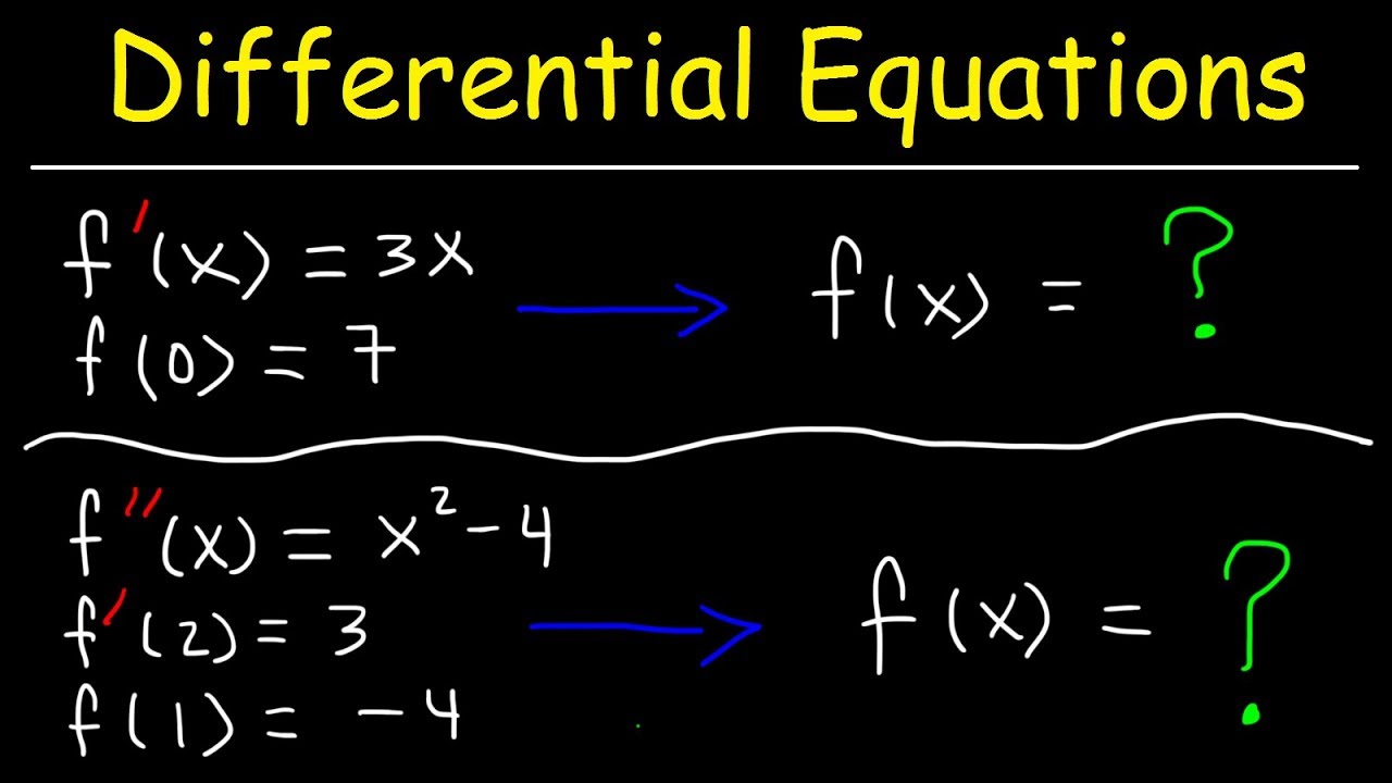
Finding Particular Solutions of Differential Equations Given Initial Conditions

Related Tags

Differential Equations Integration Method Physics Concepts Mathematical Analysis Educational Content Engineering Applications Acceleration Velocity Position Math Tutorials