How To Graph Equations - Linear, Quadratic, Cubic, Radical, & Rational Functions

The Organic Chemistry Tutor

16 Feb 201685:59

EducationalLearning

32 Likes 10 Comments

TLDRThis comprehensive video tutorial covers the fundamentals of graphing various mathematical equations, including linear, quadratic, absolute value, cubic, radical, rational, exponential, and logarithmic functions. It explains the process of plotting points, utilizing slope-intercept and standard forms, and addressing asymptotes and vertex forms for different functions. The guide also touches on the domain and range considerations for each type of function, offering a clear and detailed walkthrough for visualizing complex mathematical relationships on a graph.

Takeaways

📈 Graphing linear equations can be done using various methods such as plotting points from a table, slope-intercept form, or standard form with intercepts.
📊 For inequalities, convert the standard form to slope-intercept form for easier graphing, and use dashed lines for 'greater than' and solid lines for 'less than or equal to'.
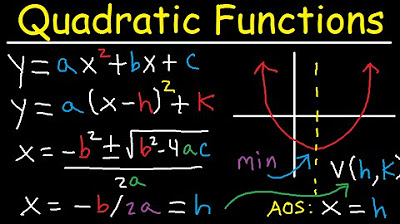
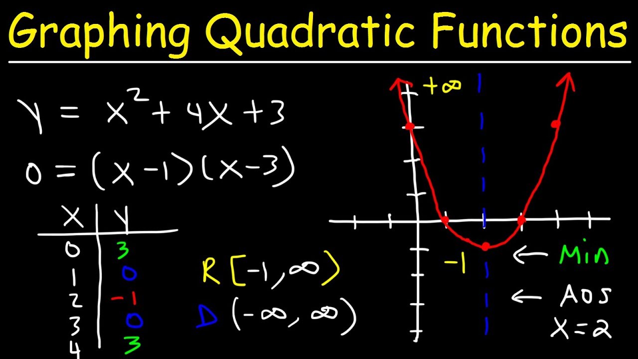
🔢 When graphing quadratic equations, finding the vertex simplifies the process, and the axis of symmetry is the x-coordinate of the vertex.
📈 Absolute value functions have a V-shape and can be graphed by considering the vertex and the direction of the slope.
📊 Cubic functions can be graphed by understanding the shifts from the origin and the direction of the function based on the sign of the coefficient.
🔢 Radical functions are graphed by shifting the origin and considering the sign of the radical and the value inside the radical.
📈 Rational functions can be graphed by identifying asymptotes and using tables to find key points that define the curve.
📊 Exponential functions have horizontal asymptotes and can be graphed by setting the exponent to zero and one to find key points.
🔢 Logarithmic functions have vertical asymptotes and can be graphed by setting the inside of the log function to one and the base to find the asymptote and key points.
📈 To graph more complex rational functions with slants or oblique asymptotes, factoring and long division can help determine the asymptote and the shape of the graph.
📊 For all functions, the domain and range are important to consider, as they define the set of possible x and y values for the graph.

Q & A

What is the first method described for graphing linear equations?
-The first method described is using a table to plot points. This involves choosing a few points by plugging in x values into the equation and finding the corresponding y values, then plotting these points on a graph and connecting them with a line.
How is the slope-intercept method used to graph linear equations?
-The slope-intercept method is used by identifying the y-intercept (b) from the equation in slope-intercept form (y = mx + b), plotting this point, and then using the slope (m) to find subsequent points by moving one unit to the right and up or down according to the slope value.
What are the steps to graph a linear equation in standard form (Ax + By = C)?
-To graph a linear equation in standard form, you find the x and y intercepts by setting y and x to zero respectively. Then, plot these intercepts and draw a line connecting them.
How do you graph inequalities involving linear equations?
-To graph inequalities, you first convert the inequality to slope-intercept form if it's in standard form. Then, plot the line representing the equation with a dashed line if the inequality is 'greater than' and a solid line if it's 'less than or equal to'. Finally, shade the correct region determined by the inequality.
What is the process for graphing quadratic equations using a data table?
-For graphing quadratic equations, you find the vertex by using the formula x = -b / 2a. Then, you choose a few x values around the vertex, calculate the corresponding y values, and plot these points on the graph. Connect the points with a smooth curve to complete the graph of the quadratic equation.
How do you convert a quadratic equation from standard form to vertex form?
-To convert a quadratic equation from standard form (ax^2 + bx + c) to vertex form (y = a(x - h)^2 + k), you complete the square by taking half of the b coefficient, squaring it, and adding it to both sides of the equation. Then, you rewrite the equation in vertex form with the vertex coordinates (h, k).
What is the general shape of a parent quadratic function in standard form?
-The general shape of a parent quadratic function in standard form (y = ax^2 + bx + c) is a parabola that opens upward if a > 0 or downward if a < 0, with the vertex at the point (h, k) where h = -b / 2a and k is the y-coordinate of the vertex.
How do you determine the domain and range of a function?
-The domain of a function is the set of all possible x-values that the function can take, while the range is the set of all possible y-values the function can produce. For linear functions, the domain is typically all real numbers, and the range is also all real numbers. For quadratic functions, the domain is all real numbers, but the range depends on whether the parabola opens upward or downward. For absolute value functions, the domain is all real numbers, and the range is from the vertex value to positive infinity.
What is the basic shape of a cubic function graph?
-The basic shape of a cubic function graph (y = ax^3 + bx^2 + cx + d) is an S-shape that can have one or two bends, depending on the coefficients. The graph can either rise from left to right or fall from left to right, and the presence of a positive or negative leading coefficient (a) determines the general direction of the curve.
How do you graph a radical function with a negative sign inside the radical?
-To graph a radical function with a negative sign inside the radical, such as y = -√(x - k), you reflect the graph of the positive radical function across the x-axis. The graph will still have a V-shape, but it will be flipped upside down compared to the positive radical function.
What is the process for graphing a rational function with a slant or oblique asymptote?
-For a rational function with a slant asymptote, where the degree of the numerator is greater than the degree of the denominator, you first factor the numerator and denominator if possible. You then find the vertical asymptotes by setting the denominator equal to zero. Since there's no horizontal asymptote, you perform long division to find the slant asymptote equation. You plot the slant asymptote with a dashed line, and then use test points to determine the shape of the graph around the asymptotes.
How do you find the horizontal asymptote of a rational function?
-To find the horizontal asymptote of a rational function, you compare the degrees of the numerator and denominator. If the degrees are equal, the horizontal asymptote is the ratio of the leading coefficients (the coefficient of the highest degree term in the numerator divided by the coefficient of the highest degree term in the denominator). If the degree of the numerator is greater than the denominator, there is no horizontal asymptote, but there is a slant or oblique asymptote.

Outlines

00:00

📈 Introduction to Graphing Equations

This paragraph introduces the concept of graphing various types of equations, including linear equations with and without inequalities, quadratic equations, transformations, radical functions, cubic functions, absolute value equations, rational expressions, exponential equations, and logarithmic equations. It begins with the basics of graphing a linear equation, such as y = 2x + 3, by plotting points and connecting them. The paragraph also discusses different methods of graphing, like using a table for linear equations and the slope-intercept method for easier visualization.

05:14

📊 Graphing Linear Equations and Inequalities

The paragraph delves into the specifics of graphing linear equations in slope-intercept form, standard form, and when they represent inequalities. It explains how to find y-intercepts, use the slope to find successive points, and connect these points to form a line. The process is demonstrated with examples, and the concept of shading regions to represent the solution sets of inequalities is introduced, with a focus on converting inequalities to slope-intercept form for easier graphing.

10:19

📈 Advanced Graphing Techniques

This section covers advanced graphing techniques for quadratic equations, absolute value functions, and cubic functions. It explains how to find the vertex of a quadratic equation, plot points around the vertex, and sketch the parabola. For absolute value functions, it describes how the graph's shape depends on the function's inside and outside signs. The paragraph also touches on cubic functions, explaining how to plot points and sketch their graphs based on the function's form and transformations.

15:20

📊 Graphing Radical Functions and Rational Expressions

The paragraph discusses the graphing of radical functions, including square roots and cube roots, and how to determine the direction of the graph based on the function's form. It explains the process of graphing rational expressions, particularly those involving the square root of x, and the importance of considering domain and range. The section also covers the impact of negative signs inside and outside the radical on the graph's orientation.

20:23

📈 Complex Rational Functions and Asymptotes

This part of the script focuses on graphing complex rational functions, including those with vertical and horizontal asymptotes. It explains how to identify and plot asymptotes, particularly for functions where the numerator's degree is higher than the denominator's, resulting in a slant or oblique asymptote. The paragraph provides a method for finding the slant asymptote through long division and emphasizes the importance of plugging in points to determine the graph's exact shape between asymptotes.

25:23

📈 Exponential and Logarithmic Functions

The final paragraph of the script covers the graphing of exponential and logarithmic functions. It explains how to find horizontal asymptotes for exponential functions and vertical asymptotes for logarithmic functions by setting the exponent or the inside of the log function to specific values. The paragraph provides examples of graphing these functions, highlighting the importance of plugging in points to connect the asymptotes and complete the graph.

Mindmap

Keywords

💡Graphing

Graphing is the process of visually representing data or functions on a coordinate plane. In the video, graphing is the primary method used to illustrate and solve various types of mathematical equations, including linear, quadratic, exponential, and logarithmic equations.

💡Linear Equations

Linear equations are mathematical equations of the form y = mx + b, where m is the slope and b is the y-intercept. These equations represent straight lines on a graph and are used to model relationships between two variables that change at a constant rate.

💡Quadratic Equations

Quadratic equations are second-degree polynomial equations of the form ax^2 + bx + c = 0. They represent parabolas on a graph and are used to model scenarios where the rate of change is proportional to the variable raised to the second power.

💡Vertex Form

Vertex form is a way of expressing a quadratic equation in the form y = a(x - h)^2 + k, where (h, k) represents the vertex of the parabola. This form makes it easy to identify the vertex and the direction in which the parabola opens.

💡Exponential Functions

Exponential functions are mathematical functions of the form y = a^x, where 'a' is a constant and 'x' is the variable. These functions describe processes that grow or decay at a rate proportional to the current value of the function.

💡Logarithmic Functions

Logarithmic functions are the inverse of exponential functions and are used to solve equations where the variable is an exponent. They have the form y = log_b(x), where 'b' is the base and 'x' is the argument of the logarithm.

💡Transformations

Transformations refer to the changes made to the graph of a function to obtain a new graph. These include shifts, stretches, reflections, and rotations. In the context of the video, transformations are used to adjust the parent functions when graphing equations like absolute value functions or equations with a different slope.

💡Inequalities

Inequalities are mathematical statements that express a relationship of inequality between two expressions, such as 'greater than' or 'less than'. They are used to describe situations where one quantity is either larger or smaller than another.

💡Standard Form

Standard form is a way of writing linear equations, typically as Ax + By = C, where A, B, and C are constants. This form is useful for finding intercepts and graphing linear equations without the need for a table of points.

💡Rational Expressions

Rational expressions are mathematical expressions that involve a numerator and a denominator, where the denominator is a variable or a function of a variable. These expressions can represent a wide range of mathematical relationships, including rates and proportions.

💡Cubic Functions

Cubic functions are polynomial functions of degree three, typically written as y = ax^3 + bx^2 + cx + d. These functions create S-shaped curves on a graph and can model a variety of phenomena with a third-degree relationship.

💡Absolute Value Equations

Absolute value equations involve the absolute value function, which takes a number as input and returns its non-negative value. These equations result in V-shaped graphs and can be used to model scenarios with constraints that are symmetric about the y-axis.

Highlights

The basics of graphing linear equations, including those with inequalities and various forms like slope-intercept and standard form.

Graphing quadratic equations by making a data table, finding the vertex, and understanding the axis of symmetry.

Transforming and graphing radical functions, including understanding the effects of the domain and range on the graph.

Cubic functions and their graphs, including identifying shifts and the behavior of the function.

Absolute value equations and their V-shaped graphs, with considerations for the slope and vertex.

Rational expressions and their graphs, including identifying vertical and horizontal asymptotes.

Exponential equations and their graphs, understanding horizontal asymptotes and key points.

Logarithmic equations and their graphs, including vertical asymptotes and the characteristics of logarithmic functions.

The process of graphing linear equations without making a table, using the slope-intercept method.

Graphing inequalities by plotting the equations in slope-intercept form and determining the correct region to shade.

The method of graphing equations in standard form by finding x and y-intercepts and connecting them.

Graphing equations with constants, such as horizontal and vertical lines.

Converting a quadratic equation from standard form to vertex form using the completing the square method.

Graphing radical functions with odd roots and understanding their symmetry properties.

The process of graphing rational functions involving a slant or oblique asymptote and the importance of factoring.

Applying the principles learned to graph new or unfamiliar equations by adapting the techniques discussed.

Transcripts

Browse More Related Video

Graphing Quadratic Functions in Vertex & Standard Form - Axis of Symmetry - Word Problems

Graphing Quadratic Functions In Standard Form Using X & Y Intercepts | Algebra

Precalculus Final Exam Review

Calculus AB Homework Day 1 - Review 1: Functions

How To Graph Functions Using an Online Calculator

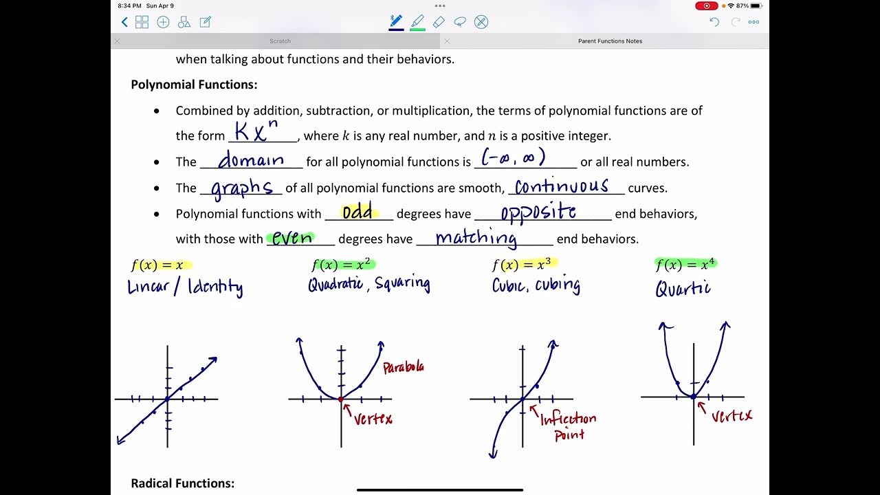
Parent Functions

Related Tags

Graphing Techniques Mathematics Tutorial Algebra Essentials Quadratic Equations Linear Equations Inequalities Graphing Exponential Functions Logarithmic Equations Educational Resource Math Skill Development