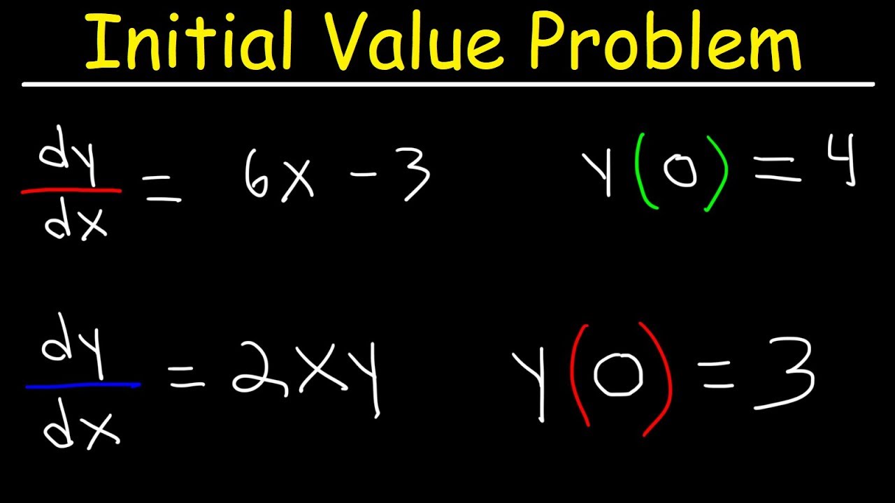
Finding Particular Solutions of Differential Equations Given Initial Conditions
TLDRThe video script demonstrates the process of solving first and second order differential equations with constant coefficients. It covers the method of integrating both sides of the equation to find the function's antiderivative and using initial conditions to solve for the constant of integration. The script provides detailed examples, including the integration process and the application of initial conditions, to arrive at particular solutions for given differential equations.
Takeaways
- 📚 To solve a differential equation, find the antiderivative of both sides to obtain the function's general form.
- 🔢 For a first-order differential equation, integrate the given function and use the initial condition to solve for the constant of integration.
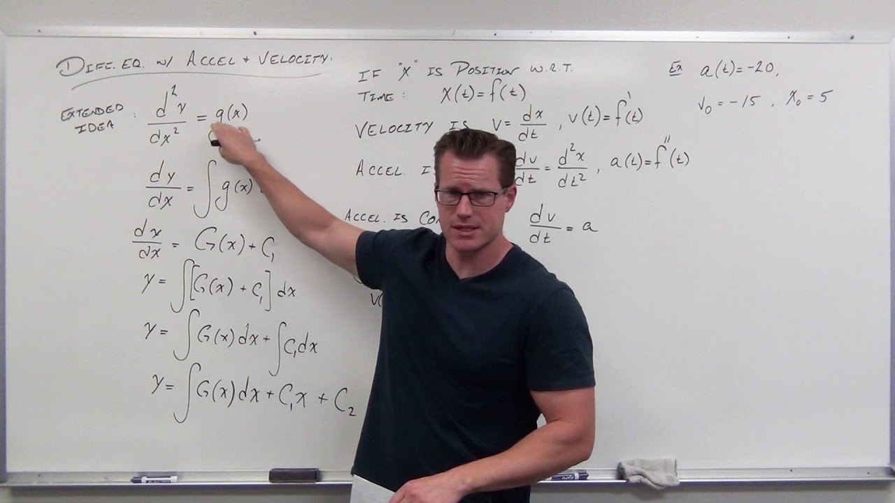
- 📈 When dealing with higher-order derivatives, multiple integrations and initial conditions may be required to find the particular solution.
- 🌟 The process of solving differential equations involves a step-by-step approach of integrating and applying initial conditions.
- 🧩 Each integration adds a new constant of integration, which must be determined using the given initial conditions.
- 📍 The initial condition provides the value of the function or its derivative at a specific point, crucial for finding the particular solution.
- 🔍 When solving second-order differential equations, you must first find the first derivative function before integrating to find the original function.
- 🛠️ The method demonstrated in the script can be applied to differential equations of any order, given enough initial conditions.
- 📊 The power rule is essential for integrating polynomial functions, where the exponent is increased by one and then divided by the new exponent.
- 🔑 The constant of integration (c) can be found by substituting the initial condition into the general solution and solving for the constant.
- 🎓 Understanding and applying the concepts of integration and initial conditions are key to solving differential equations and finding particular solutions.
Q & A
What is the given differential equation in the first example?
-The given differential equation in the first example is f'(x) = 3x.
What is the initial condition provided for the first example?
-The initial condition provided for the first example is f(0) = 7.
How does one find the antiderivative of the given differential equation?
-To find the antiderivative of the given differential equation, one integrates both sides of the equation. The antiderivative of f'(x) is f(x), and the antiderivative of 3x is (3x^2)/2 + C.
What is the particular solution to the first differential equation?
-The particular solution to the first differential equation is f(x) = (3x^2)/2 + 7.
What is the second differential equation presented in the script?
-The second differential equation presented is f''(x) = 6x^2 - 5.
What are the initial conditions for the second differential equation?
-The initial conditions for the second differential equation are f(1) = 4 and f'(1) = 2.
How does one solve a differential equation with an initial condition?
-To solve a differential equation with an initial condition, one first finds the antiderivative of the equation, then uses the initial condition to solve for the constant of integration (C).
What is the general process for solving a second-order differential equation with two initial conditions?
-The general process involves first integrating the second-order differential equation to find the first-order derivative function, then using the first initial condition to find the first constant of integration. Next, integrating the first-order derivative function to find the original function (f(x)), and finally using the second initial condition to find the second constant of integration.
What is the final form of the solution for the second differential equation example?
-The final form of the solution for the second differential equation example is f(x) = (1/3)x^3 - (5/2)x + 7.
How does the process of solving a second-order differential equation differ from a first-order one?
-The process of solving a second-order differential equation involves an additional step of integrating the second-order derivative to find the first-order derivative function, and it requires two initial conditions instead of one, as opposed to a first-order differential equation.
What is the importance of initial conditions in solving differential equations?
-Initial conditions are crucial in solving differential equations because they provide the necessary information to determine the constants of integration, which allows for a particular solution rather than a general one.
Outlines
📚 Solving First-Order Differential Equations
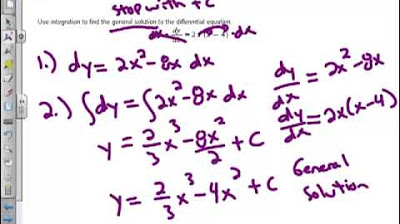
This paragraph introduces the process of solving a first-order differential equation with a given initial condition. The equation is f'(x) = 3x, and the initial condition is f(0) = 7. The explanation begins by integrating both sides of the equation to find the function f(x). The anti-derivative of f'(x) is f(x), and the anti-derivative of 3x is (3x^2)/2 + C. Using the initial condition, the constant C is determined to be 7, leading to the particular solution f(x) = (3x^2)/2 + 7. The paragraph then presents another example with a different function, f'(x) = 6x^2 - 5, and initial condition f(1) = 4, and explains the steps to find the particular solution for this case as well.
📈 Integrating Second-Order Differential Equations
This paragraph delves into solving differential equations that involve the second derivative of a function. The example provided has a second derivative of 2x - 3, and two initial conditions: f'(1) = 2 and f(0) = 3. The process starts by integrating the second derivative to find the first derivative, f'(x) = x^2 - 3x + C. Using the initial condition for the first derivative, the constant C is determined to be 4. Further integration of f'(x) yields the original function f(x) = (1/3)x^3 - (3/2)x^2 + 4x + D. Applying the initial condition for f(x), the constant D is found to be 3, thus providing the complete solution to the differential equation.
🔢 Solving with Multiple Initial Conditions
The final paragraph addresses a more complex scenario where a second derivative is given, x^2 - 4, and multiple initial conditions are provided: f'(2) = 3 and f(1) = -4. The explanation involves integrating the second derivative to obtain the first derivative, f'(x) = (1/3)x^3 - 4x + C, and then using the initial condition for f'(x) to find C = 25/3. The next step is to integrate f'(x) to get f(x), which results in f(x) = (1/12)x^4 - 2x^2 + (25/3)x + D. Applying the initial condition for f(x), D is calculated to be -125/12. The paragraph concludes with the full solution to the differential equation, f(x) = (1/12)x^4 - 2x^2 + (25/3)x - 125/12, demonstrating the method for solving equations with multiple initial conditions.
Mindmap
Keywords
💡differential equation
💡initial condition
💡antiderivative
💡integration
💡constant of integration
💡second derivative
💡power rule
💡cubic function
💡quadratic function
💡first derivative
💡integration constant
Highlights
Solving differential equations by finding the antiderivative of both sides
Given differential equation: f'(x) = 3x with initial condition f(0) = 7
Integration of f'(x) results in f(x), and the anti-derivative of 3x is (3x^2)/2 + C
Using the initial condition to solve for the constant C, resulting in f(x) = (3x^2)/2 + 7
Second example with differential equation: f'(x) = 6x^2 - 5 with initial condition f(1) = 4
Integration leads to f(x) = (6x^3)/3 - 5x + C, and solving for C using f(1) = 4 results in C = 7
Final expression for the second example: f(x) = (6x^3)/3 - 5x + 7
Handling a differential equation with the second derivative given, requiring two initial conditions
For the second derivative 2x - 3, the first derivative is x^2 - 3x + C, and solving for C using initial conditions
Deriving the function f(x) from the first derivative equation, resulting in f(x) = (1/3)x^3 - (3/2)x^2 + 4x
Third example with second derivative x^2 - 4 and initial conditions f'(2) = 3 and f(1) = -4
Integrating the first derivative expression and solving for the constant of integration using the initial conditions
Final solution for the third example: f(x) = (1/12)x^4 - 2x^2 + (25/3)x - (125/12)
The process of solving differential equations demonstrated is applicable to a variety of initial value problems
The examples provided illustrate the steps and methods for solving first and second order differential equations
Each step in solving the differential equations is clearly explained, making it a valuable resource for learning
Transcripts
Browse More Related Video
Differential Equations BC Calculus
Initial Value Problem

Separable differential equations introduction | First order differential equations | Khan Academy

Old separable differential equations introduction | Khan Academy

Simple Differential Equations
Differential Equations with Velocity and Acceleration (Differential Equations 7)
5.0 / 5 (0 votes)
Thanks for rating: