Physics - Ch 66 Ch 4 Quantum Mechanics: Schrodinger Eqn (81 of 92) Transmission Coeff., Original Eq
TLDRIn this online lecture, the presenter demonstrates how to calculate the transmission coefficient using both the original and simplified Schrödinger equations. The example uses a particle with energy of one electron volt facing a barrier of two electron volts, with a width of 500 picometers. The detailed calculation shows a slight difference between the results from the two equations, highlighting the importance of using the correct equation for accurate predictions, especially in the case of narrow barriers.
Takeaways
- 📝 The lecture focuses on calculating the transmission coefficient using both the original and simplified equations.
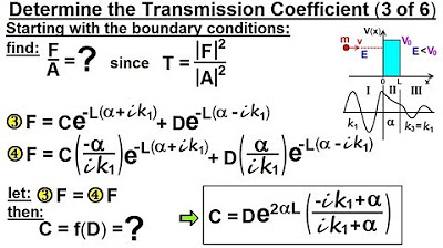
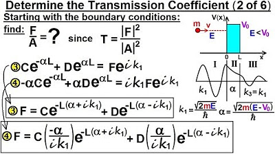
- 🔧 The original equation is derived from the Shroginger equations solved with boundary conditions.
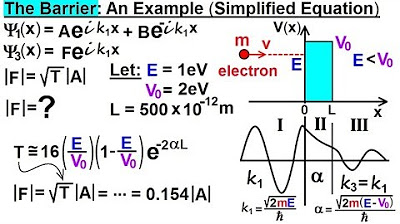
- 🌟 The simplified equation is used for quick calculations, especially when the barrier is not too wide.
- 💡 The script provides an example calculation with specific values for energy, potential, and barrier width.
- 📌 The transmission coefficient is calculated for a particle with energy of 1 eV, potential barrier of 2 eV, and barrier width of 500 picometers.
- 🧮 The calculated Alpha value, representing the decay constant in the barrier region, is 5.123 * 10^(-9).
- 🔢 The transmission coefficient using the original equation is found to be approximately 0.02355, using the hyperbolic sine function.
- 🎯 The result from the original equation is compared with a previously calculated value using the simplified equation, showing a slight difference.
- 🤔 The difference in results is noted but considered negligible for most practical purposes, with the first two decimal places matching.
- 📊 The importance of using the correct equation is emphasized, especially for very narrow barriers where the simplified version may not be accurate.
- 🚀 The process demonstrates the practical application of quantum mechanics equations in calculating particle behavior.
Q & A
What was the main topic of the lecture?
-The main topic of the lecture was calculating the transmission coefficient using both the original and simplified equations derived from Schrödinger's equations.
How many decimal places did the lecturer add to the result?
-The lecturer added one more decimal place to the result obtained from the original equation.
What were the parameters used in the example calculation?
-The parameters used were: the energy of the particle being 1 electron volt, the potential of the barrier being 2 electron volts, and the width of the barrier being 500 picometers.
What does Alpha represent in the context of this lecture?
-Alpha represents the decay constant of a particle decaying through the barrier region.
What is the formula for the transmission coefficient according to the original equation?
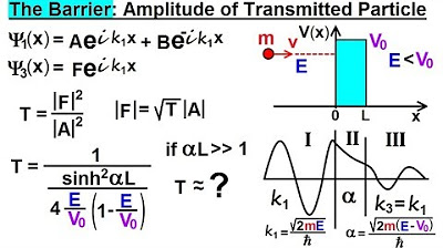
-The formula for the transmission coefficient according to the original equation is T = 1 / (1 + sinh^2(αL)), where α is the decay constant and L is the width of the barrier.
What was the calculated value of Alpha in the example?
-The calculated value of Alpha in the example was 5.123 times 10 to the power of -9.
How was the hyperbolic sine squared used in the calculation?
-The hyperbolic sine squared was used by taking the square of sinh(αL) and dividing it by the denominator in the formula for the transmission coefficient.
What was the final calculated transmission coefficient using the original equation?
-The final calculated transmission coefficient using the original equation was approximately 0.02355.
How does the simplified equation differ from the original in terms of accuracy?
-The simplified equation provides a close approximation of the transmission coefficient, but for very narrow barriers, the differences between the two equations can be quite large, necessitating the use of the original equation for greater accuracy.
What was the comparison result between the original and simplified equation calculations?
-The comparison showed that the first two decimal places were identical, but there was a difference in the third decimal place, with the original equation yielding a value of 5 and the simplified equation yielding an 8.
Why is it important to use the correct equation for calculating the transmission coefficient?
-Using the correct equation is important for accurately determining the amplitude of particle oscillations on the right side of the boundary, especially when dealing with very narrow barriers where the differences between the equations can be significant.
Outlines
🔬 Calculating Transmission Coefficient Using the Original Equation
This segment introduces the process of calculating the transmission coefficient using the original equation derived from Schrödinger's equations under certain boundary conditions. It starts by referencing a previous video where a simplified equation was used to calculate the transmission coefficient, noting the result obtained. The lecturer aims to demonstrate the calculation using the more complex original equation, emphasizing the context of a particle with an energy of one electron volt encountering a potential barrier of two electron volts with a width of 500 picometers. The goal is to determine the transmission coefficient, which involves calculating the decay constant (Alpha) through the barrier, and using it along with the particle's energy and the barrier's potential to find the transmission coefficient's value. The calculation involves the hyperbolic sine function of Alpha times the barrier's width (L), squared and added to one in the denominator of the formula for the transmission coefficient. The result, compared to the one from the simplified equation, shows slight differences but underscores that both methods yield similar values for practical purposes, with more significant disparities expected only in cases of very narrow barriers.
Mindmap
Keywords
💡Transmission Coefficient
💡Quantum Mechanics
💡Potential Barrier
💡Hyperbolic Sine
💡Boundary Conditions
💡Schrödinger Equation
💡Particle
💡Amplitude
💡Decay Constant
💡Simplified Equation
💡Tunneling
Highlights
The lecture focuses on calculating the transmission coefficient using both the original and simplified equations.
The previous video demonstrated the use of the simplified equation to calculate the transmission coefficient.
The result from the simplified equation was refined by adding an extra decimal place.
The lecture introduces the original Shroginger equation for calculating the transmission coefficient, including boundary conditions.
The energy of the particle is assumed to be one electron volt for the calculation.
The potential of the barrier is set at two electron volts.
The width of the barrier is given as 500 picometers.
The goal is to find the transmission coefficient to calculate the amplitude of oscillations on the right side of the boundary.
The value of Alpha, representing the decay constant in the barrier region, was previously calculated.
Alpha was found to be 5.123 times 10 to the power of -9.
The transmission coefficient formula involves dividing one by one plus the hyperbolic sine squared of Alpha times L.
The hyperbolic sine of Alpha times L is squared and divided by the ratio of the particle's energy to the barrier's potential.
The denominator simplifies to one, leading to the calculation of the transmission coefficient as 0.02355 using the original equation.
Comparing the result with the simplified equation, there is a slight difference in the third decimal place.
Despite the difference, the first two decimal places match, and the values are effectively the same for practical purposes.
The use of the simplified equation is recommended for very narrow barriers where differences can be significant.
The lecture concludes that the original equation must be used for wide barriers to accurately capture the transmission coefficient.
Transcripts
Browse More Related Video
Physics - Ch 66 Ch 4 Quantum Mechanics: Schrodinger Eqn (80 of 92) Transmission Coeff. Example
Physics - Ch 66 Ch 4 Quantum Mechanics: Schrodinger Eqn (78 of 92) The Barrier: Amplitude
Physics - Ch 66 Ch 4 Quantum Mechanics: Schrodinger Eqn (85 of 92) Transmission Coeff=? (3 of 6)
Physics - Ch 66 Ch 4 Quantum Mechanics: Schrodinger Eqn (84 of 92) Transmission Coeff=? (2 of 6)
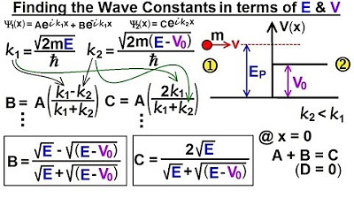
Physics - Ch 66 Ch 4 Quantum Mechanics: Schrodinger Eqn (66 of 92) B=? C=? in terms of E & V0
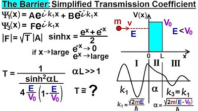
Physics - Ch 66 Ch 4 Quantum Mechanics: Schrodinger Eqn (79 of 92) Simplified Transmission Coeff.
5.0 / 5 (0 votes)
Thanks for rating: