Introduction to Statistics

The Organic Chemistry Tutor

9 Feb 202356:46

EducationalLearning

32 Likes 10 Comments

TLDRThe video provides an introduction to statistics, covering how to calculate and interpret mean, median, mode, range, quartiles, interquartile range, outliers, box plots, skewness, dot plots, stem & leaf plots, frequency tables and histograms from a dataset. It explains how to identify symmetric vs skewed distributions, construct tables to find relative frequencies and percentiles, and determine if numbers are outliers. Examples and step-by-step working are provided to demonstrate these statistical concepts and methods clearly.

Takeaways

😀 How to calculate mean, median, mode and range of a dataset
📊 How to construct a box plot and identify outliers
📈 Concepts of data skewness, positive and negative skew
🎯 How to make a stem and leaf plot and dot plot
📋 Creating frequency tables and histograms
🔢 Calculating relative and cumulative frequencies
👌 Finding percentiles from a frequency distribution
📒 Constructing frequency distribution tables
🗂️ Organizing data into classes and intervals
🖥️ Using Excel to analyze and visualize data

Q & A

How do you calculate the mean of a data set?
-To calculate the mean, take the sum of all the numbers in the data set and divide it by the total number of data points. For example, if the data set is {7, 7, 10, 14, 15, 23, 32}, the sum is 108 and there are 7 numbers. 108/7 = 15.43.
What is the difference between a bar graph and a histogram?
-A bar graph and histogram are very similar, but the bars in a histogram are adjacent to each other with no spaces in between. The bars in a bar graph are spaced out.
How do you identify if a number is an outlier in a data set?
-To identify if a number is an outlier, calculate the range using: Q1 - 1.5*IQR as the lower bound, and Q3 + 1.5*IQR as the upper bound. If a number in the data set falls outside this range, it is considered an outlier.
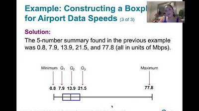
What are the key components of a box and whisker plot?
-The key components of a box and whisker plot are: the minimum, first quartile (Q1), median (second quartile/Q2), third quartile (Q3), maximum, and outliers shown as points outside the box.
How can you identify if a distribution is skewed to the left or right?
-If the shape of the data distribution has a longer tail extending to the right, it is positively or right skewed. If the tail extends further to the left, it has a negative or left skew.
What is the difference between a stem-and-leaf plot and a dot plot?
-In a stem-and-leaf plot, the data values are split into a stem digit and a leaf digit to create a tabular summary. In a dot plot, dots are used above a number line to show each data value.
What are quartiles and how are they useful?
-Quartiles divide an ordered data set into four equal groups. The first quartile (Q1) represents 25% of the data, second quartile (Q2) is 50% and third quartile (Q3) is 75%. Quartiles are useful for identifying distribution shapes and outliers.
How do you construct a frequency table?
-To construct a frequency table, list each unique data value in one column. In a second column, tally the frequency or count of occurrences for each value. Sum the frequencies to get the total number of data points.
What is relative frequency and cumulative relative frequency?
-Relative frequency is each frequency divided by the total count. Cumulative relative frequency sums the relative frequencies cumulatively to show the proportion below each data value.
What is the purpose of a stem-and-leaf plot?
-A stem-and-leaf plot organizes data by splitting each value into a stem digit and a leaf digit. This allows the shape of the distribution to be visualized and makes it easy to see clusters and gaps.

Outlines

00:00

😊 Overview of statistical concepts

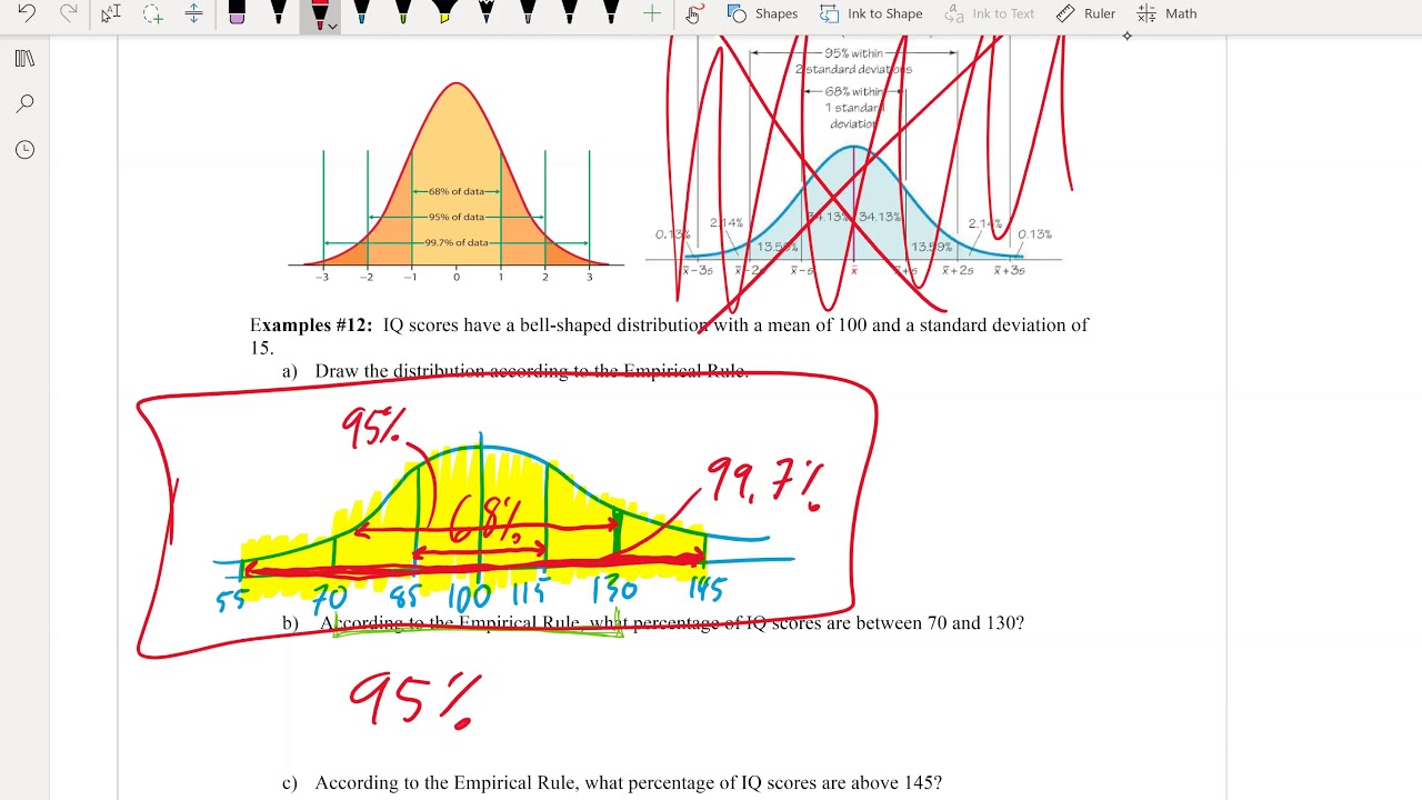
This paragraph provides an overview of key statistical concepts that will be covered, including calculating the mean, median, mode, range, quartiles, interquartile range, outliers, box plots, skewness, dot plots, stem and leaf plots, frequency tables, histograms, and relative frequencies.

05:01

😃 Calculating statistical measures

This paragraph demonstrates how to calculate the mean, median, mode, and range for two sample data sets. It explains the process step-by-step.

10:03

😃 Finding quartiles and interquartile range

This paragraph explains how to find the first, second, and third quartiles (Q1, Q2, Q3) of a data set in order to determine the interquartile range. It also shows how to identify outliers.

15:06

😃 Constructing a box plot

This paragraph discusses the components of a box plot and demonstrates how to construct one using the statistical measures calculated from a data set, including quartiles and outliers.

20:09

😃 Identifying skewed distributions

This paragraph differentiates between symmetric, positively skewed, and negatively skewed distributions. It relates skewness to the position of the mean relative to the median.

25:09

😃 Additional statistical representations

This paragraph briefly covers creating other types of statistical plots and tables, including dot plots, stem and leaf plots, frequency tables, and histograms.

30:12

😃 Using frequency tables

This paragraph shows how a frequency table summarizes a data set and can be used to efficiently calculate the mean.

35:12

😃 Constructing a stem and leaf plot

This paragraph provides two examples of creating stem and leaf plots from data sets, including plots for decimal values.

40:15

😃 Building a frequency table

This paragraph demonstrates the process of constructing a frequency table to show the distribution of values in a data set.

45:16

😃 Creating histograms

This paragraph explains the difference between histograms and bar graphs. It shows how to create a histogram using a frequency distribution table.

50:16

😃 Calculating relative frequencies

This paragraph shows how to augment a frequency table by adding columns for relative frequency and cumulative relative frequency in order to determine percentiles.

55:20

😃 Understanding percentiles visually

This paragraph explains how to determine percentiles from a cumulative relative frequency table. It also provides a visual representation to build intuition.

Mindmap

Keywords

💡Statistics

The term 'statistics' refers to the field of study focused on collecting, analyzing, interpreting, and presenting quantitative data. This entire video introduces viewers to core statistical concepts like measures of central tendency (mean, median, mode) and visualization methods (box plots, histograms etc). All the terminology and methods covered relate to describing, summarizing and making sense of numerical data.

💡Mean

The 'mean' or average is a measure of central tendency calculated by adding all data values and dividing the sum by the total number of values. The video demonstrates how to find the mean of two data sets, emphasizing that you must sum all the observations and divide by the total count.

💡Median

The median is the middle value of a dataset arranged in numerical order. As illustrated in the examples, if there are an odd number of data points, the median is the middle entry. If there are an even number, the median is the average of the two central values.

💡Mode

The mode refers to the value that appears most frequently in a dataset. The video script provides examples of identifying the mode from a set of numbers and a dot plot. A dataset can have more than one model, making it bimodal or multimodal distribution.

💡Range

The range is the difference between the maximum and minimum values in a dataset. Using two examples, the video demonstrates how to find the range by subtracting the lowest number from the highest number.

💡Quartiles

Quartiles divide a dataset into four equal groups, each representing 25% of the data. Q1, Q2, and Q3 demarcate the 4 quartiles. Q2 equals the dataset's median. Q1 and Q3 are the medians of the lower and upper halves of the data.

💡Interquartile Range

The interquartile range (IQR) measures data dispersion. It equals the difference between the third and first quartiles (Q3 - Q1). A larger IQR indicates greater spread in the data. The video example shows how to compute the IQR once the quartiles are determined.

💡Outlier

Outliers are data points that fall well outside the normal range. The video demonstrates that to identify outliers, you first compute quartiles and IQR, define a threshold range, and then detect anomalies outside this range. Anything less than Q1 - 1.5(IQR) or greater than Q3 + 1.5(IQR) is an outlier.

💡Skewness

Skewness measures the symmetry of a dataset's distribution. In a symmetrical or normal distribution with no skew, the mean equals the median. A right or positive skew exists when data clusters left with outliers on the right. The mean then exceeds the median. A left or negative skew has clustering on the right and outliers on the left. Here the median exceeds mean.

💡Histogram

Histograms visually depict the distribution of numerical data using bars, where adjacent bars touch one another. The video demonstrates creating a histogram starting with a frequency distribution table that separates scores into classes. The x-axis plots score intervals and the y-axis plots frequency count within each class.

Highlights

To find mean, median, mode, and range, first arrange data in order, then calculate each value using specific formulas.

Median is middle number when data arranged in order. Eliminate outer numbers until reach middle.

Mode is number that occurs most frequently in data set.

Range is difference between highest and lowest numbers.

To find quartiles and interquartile range, divide ordered data into 4 equal sections. Q1 and Q3 are medians of lower and upper halves.

Interquartile range (IQR) is difference between Q3 and Q1. Use to identify outliers.

Symmetrical distribution has mean = median. Skewed right distribution has mean > median. Skewed left has mean < median.

Box plots visually show quartiles and outliers. Position of Q2 indicates skewness.

Dot plots place dots above values on number line based on frequency in data set to visualize distribution.

Stem-and-leaf plots separate out digits of each number to provide overview of distribution in compact table format.

Frequency tables tally counts per unique number to enable calculations like mean.

Histograms use adjacent bars representing ranges of values to show distribution.

Relative frequency normalizes counts by total data points. Cumulative relative frequency used to find percentiles.

Percentiles identify value below which given percentage of data exists, using cumulative relative frequencies.

Visual representation shows correspondence between percentiles and location within ordered data set distribution.

Transcripts

Browse More Related Video

3.3.4 Measures of Relative Standing - Boxplots and Modified Boxplots

Elementary Stats Lesson #3 A

Math 119 Chapter 3 part 3

Live Day 2- Basic To Intermediate Statistics

How To Make Box and Whisker Plots

Plots, Outliers, and Justin Timberlake: Data Visualization Part 2: Crash Course Statistics #6