Math 14 HW 6.4.7-T Using the Central Limit Theorem
TLDRThis script explains the application of the normal distribution and the central limit theorem in statistical analysis. It walks through calculating the probability of weight gain for male college students during their freshman year, using both individual and sample mean scenarios. The process involves determining z-scores and utilizing a normal distribution calculator to find the probabilities, demonstrating the use of statistical tools in real-world data interpretation.
Takeaways
- 📊 The script discusses the normal distribution of weight gain among male college students during their freshman year, with a mean of 1.2 kg and a standard deviation of 5.3 kg.
- 🔍 Part A of the script involves calculating the probability of a randomly selected male college student gaining between 0 kg and 3 kg during their freshman year.
- 📈 The script explains the use of a bell curve to represent the normal distribution and how to find the area under the curve for a given range of values.
- 📝 The process of finding z-scores for the values 0 kg and 3 kg is described, which involves subtracting the mean from the value and dividing by the standard deviation.
- 🧮 The first z-score is calculated to be -0.23, and the second z-score is 0.34, which are then used to find the probability using a statistical calculator.
- 📉 The script uses StatCrunch to find the probability between the two z-scores, resulting in a probability of 0.2240 for one student.
- 👥 Part B of the script addresses the probability of the mean weight gain of a sample of nine male college students being between 0 kg and 3 kg.
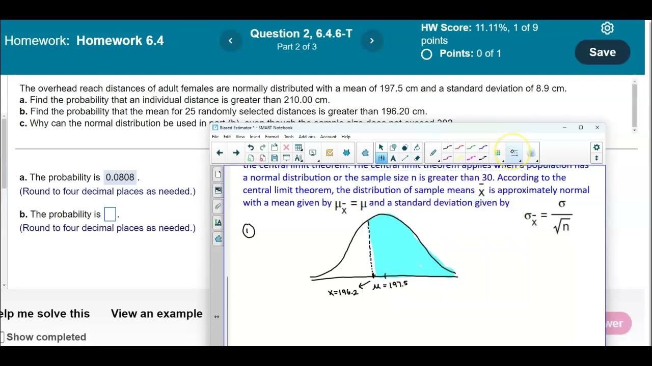
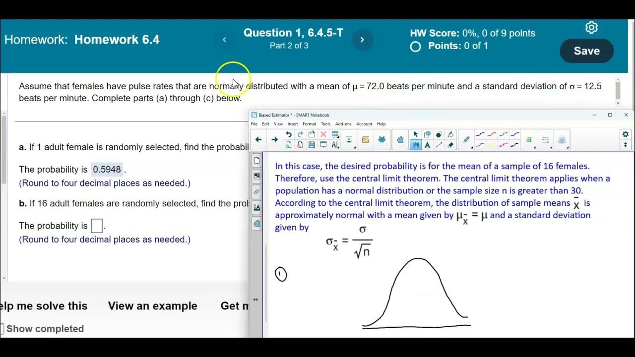
- 📚 The Central Limit Theorem is introduced, which allows for the use of the normal distribution to approximate the distribution of sample means even when the sample size is less than 30.
- 🔄 The standard deviation of the sample means is calculated by dividing the population standard deviation by the square root of the sample size (5.3 / √9).
- 📐 New z-scores are calculated for the sample mean scenario, resulting in -0.68 and 1.02, which are then used to find the probability for the sample of nine students.
- 📊 Using StatCrunch again, the probability for the sample mean of nine students is found to be 0.5979.
- ❓ The script concludes with a question about the applicability of the normal distribution in Part B, explaining that it is valid due to the original population being normally distributed.
Q & A
What is the normal distribution assumption for the weight gain of male college students during their freshman year?
-The weight gain of male college students during their freshman year is assumed to be normally distributed with a mean of 1.2 kilograms and a standard deviation of 5.3 kilograms.
What is the probability that a randomly selected male college student gains between zero and three kilograms during their freshman year?
-To find this probability, the script calculates the z-scores for 0 and 3 kilograms and then uses a normal distribution calculator to find the area under the curve between these z-scores, resulting in a probability of 0.2240.
How does one calculate the z-score for a given value in a normal distribution?
-The z-score is calculated by subtracting the mean from the given value and then dividing by the standard deviation. For example, for a value of 0 kilograms, the z-score is (0 - 1.2) / 5.3, which is approximately -0.23.
What is the purpose of using StatCrunch in this context?
-StatCrunch is used to calculate the probability that corresponds to a given z-score in a normal distribution, which helps in finding the area under the curve between two z-scores.
What is the Central Limit Theorem and how does it apply to this scenario?
-The Central Limit Theorem states that the distribution of sample means will be approximately normal for any sample size, provided the original population is normally distributed. In this case, it is used to calculate the probability for the mean weight gain of nine male college students.
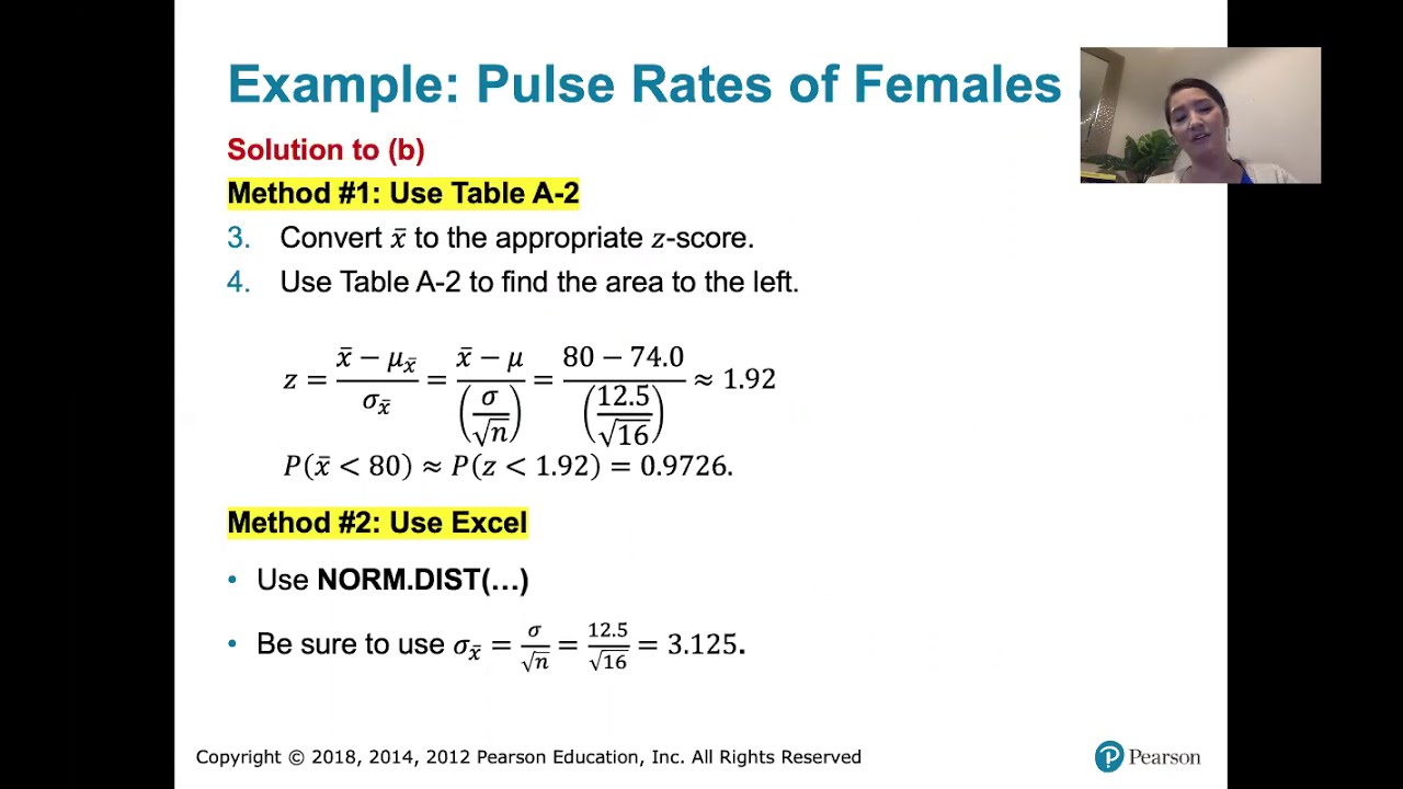
How is the standard deviation of the sample means calculated when using the Central Limit Theorem?
-The standard deviation of the sample means is calculated by dividing the population standard deviation by the square root of the sample size (n). In this case, it is 5.3 / sqrt(9).
What is the probability that the mean weight gain of nine randomly selected male college students is between zero and three kilograms?
-The script calculates the z-scores for the sample means of 0 and 3 kilograms and then uses StatCrunch to find the area under the curve, resulting in a probability of 0.5979.
Why can the normal distribution be used in Part B even though the sample size does not exceed 30?
-The normal distribution can be used because the original population is normally distributed, and according to the Central Limit Theorem, the distribution of the sample means is a normal distribution for any sample size.
What is the significance of the bell curve in this context?
-The bell curve represents the normal distribution of the weight gain. It helps visualize the distribution and the areas corresponding to different probabilities, which is essential for calculating the probabilities in the script.
What is the difference between calculating an individual's weight gain probability and the mean weight gain probability for a group?
-Calculating an individual's weight gain probability involves finding the z-score for the individual's weight gain and looking up the corresponding probability in a normal distribution table. For a group, especially when using the Central Limit Theorem, one calculates the z-scores for the mean of the group's weight gain and finds the probability for the mean of the sample means.
Outlines
📊 Calculating Freshman Weight Gain Probability
This paragraph discusses the statistical approach to determine the probability of a male college student gaining between zero and three kilograms during their freshman year, assuming a normal distribution with a mean of 1.2 kg and a standard deviation of 5.3 kg. The process involves sketching a bell curve, identifying the mean and standard deviation, and calculating z-scores for the specified weight gain intervals. The z-scores for 0 kg and 3 kg are calculated to be -0.23 and 0.34, respectively, and a statistical tool like StatCrunch is used to find the probability of the area under the curve between these z-scores, resulting in a probability of 0.2240.
📚 Applying the Central Limit Theorem for Sample Means
The second paragraph extends the analysis to a sample of nine male college students, aiming to find the probability that their average weight gain falls between zero and three kilograms. Utilizing the Central Limit Theorem, which is applicable due to the normal distribution of the population or a sample size greater than 30, the distribution of sample means is considered normal. The mean and standard deviation for the sample means are calculated, and new z-scores for the sample mean range are determined to be -0.68 and 1.02. StatCrunch is again used to compute the probability between these z-scores, yielding a result of 0.5979, indicating the likelihood of the sample mean falling within the specified range.
🤔 Rationale for Using Normal Distribution in Part B
The final paragraph addresses a question about the applicability of the normal distribution in Part B, even though the sample size does not exceed 30. It clarifies that the normal distribution can be used for the sample means because the original population is normally distributed, and thus the distribution of sample means is also normal for any sample size, not just those greater than 30. The answer to the question is provided as 'D', indicating that the normal distribution is indeed appropriate for this scenario.
Mindmap
Keywords
💡Normal Distribution
💡Mean
💡Standard Deviation
💡Z-Score
💡Probability
💡Bell Curve
💡Central Limit Theorem
💡Sample Size
💡StatCrunch
💡Area Under the Curve
Highlights
Assumption of normally distributed weight gain among male college students during their freshman year.
Mean weight gain is 1.2 kilograms with a standard deviation of 5.3 kilograms.
Using the normal distribution to find the probability of weight gain between 0 and 3 kilograms.
Graphical representation of the normal distribution curve with mean and standard deviation.
Calculation of z-scores for the given weight gain range using the formula (X - mean) / standard deviation.
First z-score calculation results in -0.23 for weight gain of 0 kilograms.
Second z-score calculation results in 0.34 for weight gain of 3 kilograms.
Utilization of StatCrunch software to find the probability between z-scores.
Probability calculation yields a result of 0.2240 for an individual student.
Application of the Central Limit Theorem for a sample size of nine students.
Adjustment of the standard deviation for sample means using the formula (standard deviation / √n).
New z-scores calculated for the sample mean weight gain scenario.
Z-score results are -0.68 for a sample mean of 0 kilograms and 1.02 for 3 kilograms.
Re-calculation of probability using StatCrunch for the sample mean scenario.
Probability result for the sample mean weight gain is 0.5979.
Explanation of why the normal distribution can be used in Part B despite the sample size not exceeding 30.
The normal distribution of the original population allows for the use of the Central Limit Theorem regardless of sample size.
Transcripts
Browse More Related Video


5.0 / 5 (0 votes)
Thanks for rating: