Calculating the area of Deadweight Loss (welfare loss) in a Linear Demand and Supply model
TLDRThis educational video teaches viewers how to calculate the area of deadweight loss in a market when it's not at equilibrium. Starting with equilibrium price and quantity, the script demonstrates how to find consumer and producer surplus, then shifts to a non-equilibrium scenario at a higher price. It illustrates the decrease in consumer surplus and increase in producer surplus, leading to a total welfare calculation. The script concludes by showing the loss in total welfare, equating to a deadweight loss, and offers an alternative method for calculating this loss using the areas of two triangles.
Takeaways
- 📈 The video explains how to calculate the area of deadweight loss in a market with a linear demand and supply graph when the market price deviates from the equilibrium price.
- 📚 Viewers should be familiar with deriving demand and supply equations from data and graphing them before watching this video.
- 📉 The script provides a step-by-step guide to plotting demand and supply curves on a graph using derived equations.
- 💰 The equilibrium price and quantity for olives in the example are $5 and 20,000 kilograms, respectively.
- 🔍 To find consumer and producer surplus at equilibrium, the script describes calculating the area of two triangles formed by the demand and supply curves.
- 📊 Consumer surplus is the area above the equilibrium price and under the demand curve, while producer surplus is the area below the equilibrium price and above the supply curve.
- 📉 At a price higher than equilibrium (e.g., $7), consumer surplus decreases, and producer surplus increases, affecting total welfare.
- 🧩 The script breaks down the calculation of producer surplus into a rectangle and a triangle to simplify the process.
- 📌 At a price of $7, total welfare is calculated by adding the reduced consumer surplus ($10) to the increased producer surplus ($50), resulting in $60.
- 🔑 Deadweight loss is determined by comparing total welfare at disequilibrium to that at equilibrium, resulting in a loss of $20,000 in the example.
- 📝 An alternative method to find deadweight loss is by calculating the area of the two triangles representing the loss of consumer and producer surplus.
Q & A
What is the main topic of the video script?
-The main topic of the video script is how to calculate the area of deadweight loss in a market when there is a deviation from the equilibrium price and quantity in a linear demand and supply graph.
What are the prerequisites for understanding the video content?
-The prerequisites for understanding the video content include familiarity with deriving demand and supply equations from data, graphing those equations, and understanding how to calculate consumer and producer surplus in a linear demand and supply model.
What is the equilibrium price and quantity of olives according to the graph in the script?
-The equilibrium price of olives is $5, and the equilibrium quantity is 20,000 kilograms.
How is consumer surplus represented on a demand and supply graph?
-Consumer surplus is represented by the area above the equilibrium price and below the demand curve on a demand and supply graph.
What is the formula for calculating the area of consumer surplus when the market is at equilibrium?
-The area of consumer surplus at equilibrium is calculated as the area of a triangle, which is 0.5 * base * height, where the base is the equilibrium quantity and the height is the difference between the demand price and the equilibrium price.
How is producer surplus represented on a demand and supply graph?
-Producer surplus is represented by the area below the equilibrium price and above the supply curve on a demand and supply graph.
What happens to consumer surplus when the market price is higher than the equilibrium price?
-When the market price is higher than the equilibrium price, the area of consumer surplus decreases because consumers are willing and able to buy fewer goods at the higher price, resulting in less consumer surplus.
How does the producer surplus change when the market price is higher than the equilibrium price?
-Producer surplus can increase when the market price is higher than the equilibrium price because producers are able to sell their goods at a higher price, but the increase may be offset by a decrease in the quantity demanded.
What is the total welfare when the market is at equilibrium, according to the script?
-The total welfare when the market is at equilibrium is $80, which is the sum of consumer surplus ($40) and producer surplus ($40).
How is the deadweight loss calculated when the market is in disequilibrium?
-Deadweight loss is calculated by finding the difference in total welfare between the equilibrium and disequilibrium states. It represents the loss of total welfare due to the market not being at its most efficient point.
What is the total welfare at the disequilibrium price of $7 in the script?
-The total welfare at the disequilibrium price of $7 is $60, which is the sum of consumer surplus ($10) and producer surplus ($50).
How much is the deadweight loss when the market price is $7, as per the script?
-The deadweight loss when the market price is $7 is $20,000, which is the difference between the total welfare at equilibrium ($80,000) and the total welfare at the disequilibrium price ($60,000).
Outlines
📊 Calculating Deadweight Loss in Market Disequilibrium
This paragraph introduces the concept of calculating deadweight loss in a market scenario where the price deviates from the equilibrium. The script explains the prerequisites, such as understanding the derivation of demand and supply equations and the ability to graph them. It sets the stage for a detailed explanation of how to calculate consumer and producer surplus and the total welfare at equilibrium, using the example of olives. The equilibrium price and quantity are identified as $5 and 20,000 kilograms, respectively. The paragraph concludes with a teaser for the upcoming calculation of deadweight loss when the market is not at equilibrium.
📉 Impact of Price Changes on Consumer and Producer Surplus
The second paragraph delves into the effects of a non-equilibrium market price on consumer and producer surplus. It uses the example of olives priced at $7 instead of the equilibrium $5. The script explains how higher prices reduce consumer surplus and increase producer surplus, but with fewer producers able to sell due to decreased demand. The calculation of consumer surplus at the higher price is straightforward, resulting in a decrease to $10. For producer surplus, the script describes a more complex calculation involving both a rectangle and a triangle, resulting in an increase to $50. The total welfare at the higher price is $60, which is less than the equilibrium welfare of $80, indicating a loss in total welfare of $20,000. The paragraph also introduces the concept of deadweight loss as the inefficiency resulting from market disequilibrium, which is calculated by subtracting the new total welfare from the equilibrium welfare.
Mindmap
Keywords
💡Deadweight Loss
💡Linear Demand and Supply Graph
💡Equilibrium Price and Quantity
💡Consumer Surplus
💡Producer Surplus
💡Disequilibrium
💡Total Welfare
💡Demand and Supply Equations
💡Market Inefficiency
💡Right Triangles
💡Supply Schedule
Highlights
Introduction to calculating the area of deadweight loss in a linear demand and supply graph when the market is not at equilibrium.
Assumption that viewers are familiar with deriving demand and supply equations and graphing them.
Presentation of a demand and supply schedule for olives with price ranges and corresponding quantities.
Derivation of demand and supply equations from the data provided in the schedule.
Graphical representation of the derived demand and supply curves on a graph.
Identification of the equilibrium price and quantity for olives as $5 and 20,000 kilograms respectively.
Explanation of calculating consumer and producer surplus at equilibrium as areas of triangles.
Calculation of total welfare in the market at equilibrium as the sum of consumer and producer surplus.
Impact of market disequilibrium on consumer and producer surplus, with a shift in price from $5 to $7.
Reduction in consumer surplus due to a higher market price.
Increase in producer surplus due to the higher selling price, despite reduced quantity sold.
Calculation of the new consumer surplus at the non-equilibrium price of $7.
Complex calculation of producer surplus involving both a rectangle and a triangle area.
Determination of total welfare at the disequilibrium price, showing a decrease from the equilibrium state.
Introduction to the concept of deadweight loss as a measure of market inefficiency.
Methodology to calculate deadweight loss by comparing total welfare at equilibrium and disequilibrium.
Visual representation of deadweight loss as two triangles on the graph.
Alternative method to calculate deadweight loss by directly finding the area of the two triangles.
Conclusion emphasizing the importance of understanding deadweight loss in economic analysis.
Special acknowledgment of a student's achievement in the class.
Transcripts
Browse More Related Video
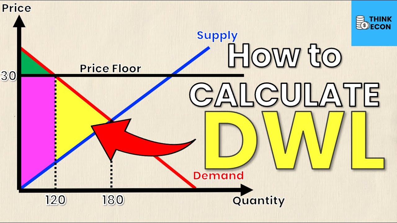
How to Calculate Deadweight Loss (with a Price Floor) | Think Econ
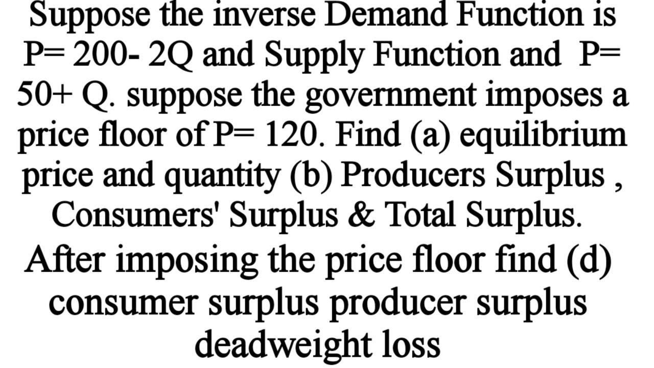
Consumers 'surplus Producers' Surplus , Total surplus, deadweight loss with price floor
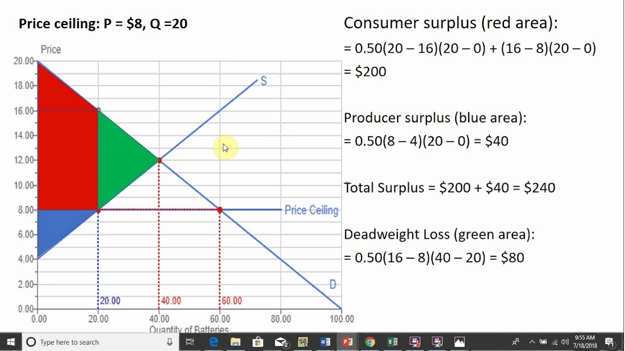
Price Ceiling: Consumer Surplus, Producer Surplus, & Deadweight loss

Rent Control and Deadweight Loss
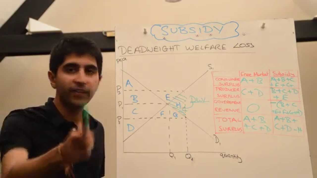
Y1/IB 29) Subsidy and Deadweight Welfare Loss

Consumer Surplus and Producer Surplus
5.0 / 5 (0 votes)
Thanks for rating: