Elementary Statistics - Chapter 5 Binomial Distributions Part 2

Joan DeRosa

24 Sept 201724:10

EducationalLearning

32 Likes 10 Comments

TLDRThis video script delves into the concept of binomial distributions, explaining the conditions required for an experiment to be classified as binomial, including fixed number of trials, two possible outcomes, and constant probability of success. It provides examples of binomial experiments, such as a surgical procedure's success rate, and illustrates how to calculate probabilities using a calculator. The script also covers how to create a binomial distribution table and calculate mean, variance, and standard deviation for binomial scenarios, offering a comprehensive guide to understanding and applying binomial distributions.

Takeaways

📐 A binomial experiment has two possible outcomes, success or failure, with 'success' not necessarily being positive.
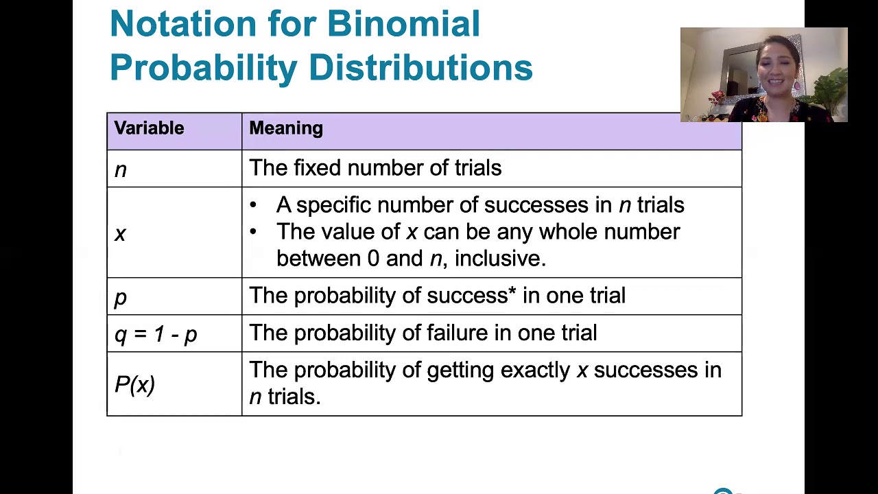
🔢 The number of observations in a binomial experiment is fixed and denoted by 'n'.
🎲 Observations in a binomial experiment are independent, meaning the outcome of one does not affect the others.
💡 The probability of success (P) is constant across all observations in a binomial experiment.
⚖️ To find the probability of failure (Q), subtract the probability of success (P) from 1.
📊 The random variable (X) in a binomial experiment ranges from 0 to the number of trials (n).
👨‍⚕️ An example given is a surgical procedure with an 85% success rate performed on 8 patients, fitting the binomial experiment criteria.
🚫 An example of a non-binomial experiment is drawing marbles from a jar without replacement, as it changes the probability with each draw.
📉 The probability of failure (Q) is crucial for calculating the binomial distribution and can be found using Q = 1 - P.
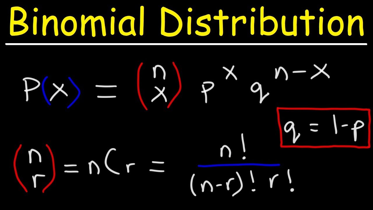
📈 Binomial probability can be calculated using a formula involving combinations, success rate, and failure rate, or with a calculator.
📊 Creating a binomial distribution table involves listing the random variables and their corresponding probabilities, which can be found using a calculator.

Q & A

What are the four conditions required for an experiment to be considered a binomial experiment?
-The four conditions are: 1) Each observation falls into one of two categories, success or failure. 2) There is a fixed number of observations, denoted by n. 3) The observations must be independent of each other. 4) The probability of success, P, is the same for each observation.
How is the probability of failure, Q, related to the probability of success, P, in a binomial experiment?
-The probability of failure, Q, is found by subtracting the probability of success, P, from one: Q = 1 - P.
What does the random variable X represent in a binomial experiment?
-The random variable X represents the number of successes in the trials of a binomial experiment, starting from 0 up to the number of trials, n.
In the context of the surgical procedure example, what is the value of n, and what does it represent?
-In the surgical procedure example, n is 8, representing the number of patients the doctor performs the procedure on.
How does the presence of different colored marbles in a jar affect the binomial experiment if marbles are drawn without replacement?
-Drawing marbles without replacement changes the probability of drawing a red marble with each subsequent draw, making the experiment not binomial because the probability is not the same for each trial.
What is the probability of success for women in the United States considering reading as their favorite leisure time activity, according to the 'pause and try' example?
-The probability of success for women considering reading as their favorite leisure time activity is 41%.
How can you calculate the probability of a binomial experiment using a calculator?
-You can calculate the binomial probability using a calculator by entering the number of trials (n), the probability of success (P), and the number of successes (x), then using the binomial distribution function (often labeled as 'binompdf' or 'bi n Oh M' on some calculators).
What is the formula used to calculate the binomial probability, and what does it involve?
-The binomial probability formula involves the combination formula, the probability of success (P), and the probability of failure (Q). It calculates the probability of obtaining a certain number of successes in a fixed number of trials.
How can you create a binomial distribution table for a given scenario?
-To create a binomial distribution table, you list the possible values of the random variable (from 0 to n) and calculate the probability for each using the binomial probability formula or a calculator, then fill in the table with these probabilities.
What does it mean to find the probability of 'at least' a certain number of successes in a binomial experiment?
-Finding the probability of 'at least' a certain number of successes involves summing the probabilities of that number of successes and all higher values of the random variable.
How are the mean, variance, and standard deviation of a binomial distribution calculated?
-The mean is calculated as the number of trials (n) multiplied by the probability of success (P). The variance is calculated as n times P times Q (1-P). The standard deviation is the square root of the variance.

Outlines

00:00

🔍 Understanding Binomial Experiments and Their Conditions

This paragraph introduces the concept of binomial experiments, which are characterized by having exactly two possible outcomes: success or failure. It emphasizes that success is not necessarily positive and provides an example involving people getting colds after being doused with water. The conditions for a binomial experiment include a fixed number of observations (n), independence of observations, and a constant probability of success (P) for each observation. The paragraph also explains the notation used for binomial experiments, including how to represent the number of trials, the probability of success and failure, and the random variable (X) that ranges from 0 to n.

05:02

📚 Applying the Binomial Experiment Framework to Real-World Scenarios

The second paragraph delves into applying the binomial experiment framework to various scenarios, such as a surgical procedure with an 85% success rate performed on eight patients and a marble-drawing experiment. It explains how to identify the number of trials (n), the probability of success (P), the probability of failure (Q, calculated as 1 - P), and the range of the random variable (X). The paragraph highlights the importance of the conditions for a binomial experiment, such as the fixed number of trials and the independence and constant probability of each trial, using examples to illustrate when a scenario does not fit the binomial model.

10:03

🧮 Calculating Binomial Probabilities Using a Calculator

This paragraph instructs how to use a calculator, specifically a Texas Instrument 83 or 84, to calculate binomial probabilities. It provides a step-by-step guide on navigating the calculator's menu to access the binomial distribution function (binomPDF) and input the necessary parameters: the number of trials (n), the probability of success (P), and the number of successes (x). The paragraph also discusses an example involving a knee surgery with a 75% success rate performed on three patients, demonstrating how to calculate the probability of exactly two successful surgeries using the calculator.

15:07

📊 Creating a Binomial Distribution Table for Survey Data

The fourth paragraph focuses on creating a binomial distribution table using survey data as an example. It outlines the process of extracting key information such as the sample size (n), the probability of success (P), and the range of random variables (X). The paragraph explains how to use a calculator to find the probability for each random variable and fill out the distribution table. It also addresses the importance of interpreting scientific notation correctly when reading probabilities from the calculator.

20:10

📉 Summing Probabilities for 'At Least' and 'More Than' Scenarios

The final paragraph discusses how to calculate the probability of 'at least' or 'more than' a certain number of successes in a binomial distribution. It uses examples involving surveys to illustrate the process of summing the probabilities for the desired range of random variables. The paragraph emphasizes the importance of including or excluding the lower bound of the range based on the specific question being asked and demonstrates how to find the sum of probabilities for different scenarios, such as at least two or more than two successes.

📏 Calculating Mean, Variance, and Standard Deviation for Binomial Distributions

This paragraph explains the mathematical concepts of mean, variance, and standard deviation in the context of binomial distributions. It provides formulas for calculating these statistical measures and illustrates their application with examples, such as the number of cloudy days in a month. The paragraph shows how to multiply the number of trials by the probability of success to find the mean, how to calculate variance by considering the product of the number of trials, the probability of success, and the probability of failure, and how to find the standard deviation by taking the square root of the variance.

Mindmap

Keywords

💡Binomial Distribution

Binomial Distribution is a probability distribution that describes the number of successes in a fixed number of independent Bernoulli trials with the same probability of success. In the video, it is the central theme, used to explain the outcomes of experiments with two possible results, such as the number of people getting colds after being doused with water.

💡Success and Failure

In the context of binomial experiments, 'success' and 'failure' are the two possible outcomes of each observation. The video emphasizes that success is not necessarily positive, as illustrated by defining getting a cold as a 'success' in one experiment, to highlight that it's just one of the two categories being measured.

💡Fixed Number of Observations

This concept refers to the constant number of trials or observations in a binomial experiment, denoted by 'n'. The video script explains that for a binomial experiment to be valid, there must be a fixed number of observations that are independent of each other.

💡Independence

Independence in the script means that the result of one observation does not affect the results of the others. This is a key condition for binomial experiments, ensuring that the probability of success remains the same for each trial, as illustrated in the examples of the surgical procedure and marble drawing.

💡Probability of Success (P)

The 'probability of success', denoted by 'P', is the chance that a single trial will result in a success. The video explains how this is a constant value for all trials in a binomial experiment, such as the 85 percent success rate of a surgical procedure.

💡Probability of Failure (Q)

The 'probability of failure', represented by 'Q', is calculated as 1 - P and represents the likelihood of an observation resulting in failure. The script uses this concept to demonstrate how to find the failure probability when the success probability is known, such as subtracting the 85 percent success rate from 1 to get 15 percent failure rate.

💡Random Variable (X)

The 'random variable', denoted by 'X', is the variable that represents the number of successes in a binomial experiment. The video script explains that it ranges from 0 to the number of trials, 'n', and is used to calculate probabilities of different outcomes, such as the number of red marbles drawn from a jar.

💡Binomial Experiment

A 'binomial experiment' is an experiment that meets the conditions of having two possible outcomes, a fixed number of trials, independence of trials, and equal probability of success for each trial. The script provides several examples, including the surgical procedure and the marble drawing, to illustrate what constitutes a binomial experiment.

💡Complement of a Probability

The 'complement of a probability' is the probability that an event will not occur, calculated as 1 minus the probability of the event. The video script explains this concept when discussing how to find the probability of failure (Q) from the probability of success (P).

💡Binomial Probability Formula

The 'binomial probability formula' is used to calculate the probability of a given number of successes in a binomial experiment. The script describes the formula's components, including the trial size (n), the probability of success (P), and the number of successes (X), and how it is applied to find specific probabilities, such as the probability of a surgical procedure being successful on exactly two patients.

Highlights

Binomial experiments require two possible outcomes: success or failure, with success not necessarily being positive.

A fixed number of observations (n) is essential for binomial experiments, with each observation being independent.

The probability of success (P) remains constant across all observations in a binomial experiment.

The probability of failure (Q) is calculated as 1 - P.

Random variables in binomial experiments are represented by X, ranging from 0 to the number of trials (n).

The binomial distribution is used to model the number of successes in a fixed number of independent trials.

An example of a binomial experiment is a surgical procedure with an 85% success rate performed on 8 patients.

Binomial experiments are not applicable when observations are not independent, such as drawing without replacement.

The probability of success for a binomial experiment can be determined using a calculator's binomial distribution function.

The binomial probability formula involves combinations and the probabilities of success and failure.

Creating a binomial distribution table involves calculating probabilities for each possible outcome.

The mean, variance, and standard deviation of a binomial distribution can be calculated using the number of trials and the probability of success.

The mean of a binomial distribution is the product of the number of trials and the probability of success.

Variance in a binomial distribution is calculated as the number of trials multiplied by the product of the probabilities of success and failure.

The standard deviation of a binomial distribution is the square root of the variance.

Practical examples of binomial distribution include determining the number of cloudy days in a month or the number of people trusting newspapers.

Summing probabilities in a binomial distribution can be used to find the likelihood of at least a certain number of successes.

Understanding scientific notation is crucial when interpreting probabilities from a calculator in binomial distribution.

Transcripts

Browse More Related Video

Math 119 Chapter 5 part 2

The Binomial Experiment and the Binomial Formula (6.5)

5.2.1 Binomial Probability Distributions - Is this procedure described by a binomial distribution?

Finding The Probability of a Binomial Distribution Plus Mean & Standard Deviation

Types Of Distribution In Statistics | Probability Distribution Explained | Statistics | Simplilearn

Binomial Distribution EXPLAINED in UNDER 15 MINUTES!

Related Tags

Binomial Distribution Statistical Experiments Probability Theory Success-Failure Observational Studies Mathematical Modeling Data Analysis Random Variables Calculus Applications Educational Content Probability Calculations