Math 119 Chapter 5 part 2
TLDRThis educational video script covers the second half of chapter five, focusing on the binomial probability distribution. It explains the concept, suitable for discrete events with two outcomes, and outlines the requirements for binomial distribution, including a fixed number of trials, independence, and two possible outcomes labeled as success or failure. The script provides examples, such as flipping a coin and selecting jurors, to illustrate how to calculate probabilities using the binomial formula and a calculator. It also discusses how to find the mean, variance, and standard deviation for binomial distributions, emphasizing the use of shortcuts for these calculations. The importance of understanding these concepts for exams is highlighted.
Takeaways
- 📚 The lesson covers the second half of chapter five, focusing on the binomial probability distribution, a discrete probability distribution for situations with two possible outcomes.
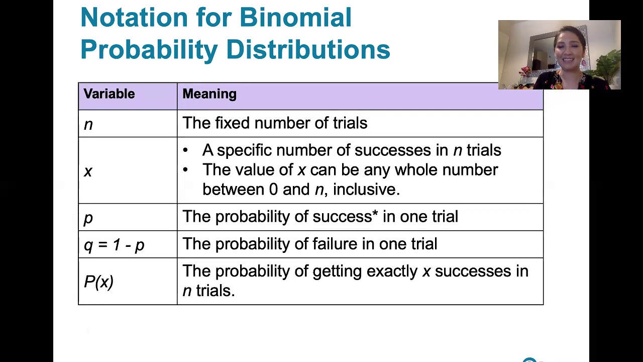
- 🎯 The binomial distribution is characterized by a fixed number of trials (n), independent events, two possible outcomes (success/failure), and the same probability of success (p) for each trial.
- 🔄 Success and failure are not about good or bad but represent the outcomes of interest and those that are not, respectively.
- 🧩 The probability of failure (q) is the complement of the probability of success, calculated as 1 - p.
- 🪙 Examples given include coin flips, blood type inheritance, and juror selection, all illustrating the application of the binomial distribution in various scenarios.
- 📉 The binomial random variable (x) represents the number of successes observed in the trials, and x can range from 0 to n.
- 📊 The binomial probability formula is introduced for calculating the probability of exactly x successes in n trials, but it's recommended to use a calculator for such calculations.
- 🔢 The script emphasizes the use of a calculator for finding binomial probabilities, using functions like 'binomial pdf' for exact probabilities and 'binomial cdf' for cumulative probabilities.
- 📈 Mean (μ), variance, and standard deviation for a binomial distribution can be quickly calculated using shortcuts: mean = n * p, variance = n * p * q, and standard deviation = √(variance).
- 🤔 The concept of 'usual' values is discussed, using the mean ± 2 standard deviations as a rule of thumb to determine if a result is unusual within a binomial distribution.
- 📝 The importance of understanding both the manual calculations and the use of technology (calculators) is highlighted for solving binomial distribution problems efficiently.
Q & A
What is the main topic discussed in the video script?
-The main topic discussed in the video script is the binomial probability distribution, which is a discrete probability distribution that allows for only two possible outcomes of an event.
What are the four key characteristics of a binomial probability distribution as outlined in the script?
-The four key characteristics of a binomial probability distribution are: 1) a fixed number of trials (n), 2) the trials are independent events, 3) each trial has an outcome classified as either success (p) or failure (q), and 4) the probability of success is the same for each trial.
What does the term 'success' represent in the context of binomial probability distribution?
-In the context of binomial probability distribution, 'success' represents the outcome that the researcher or experimenter is looking for, and it does not necessarily imply a positive or good outcome. It is one of the two possible outcomes, the other being 'failure'.
How is the probability of failure (q) related to the probability of success (p) in a binomial distribution?
-The probability of failure (q) is the complement of the probability of success (p). This means that q is equal to 1 - p.
What is the binomial random variable x in the context of the video script?
-In the context of the video script, the binomial random variable x represents the number of successes observed in the fixed number of independent trials.
Can you explain the example given in the script about flipping a fair coin?
-The example of flipping a fair coin illustrates a binomial experiment where the coin is flipped 10 times (fixed number of trials, n=10). The outcomes are independent, and each flip has two possible outcomes: heads (success) or tails (failure), each with a probability of 0.5.
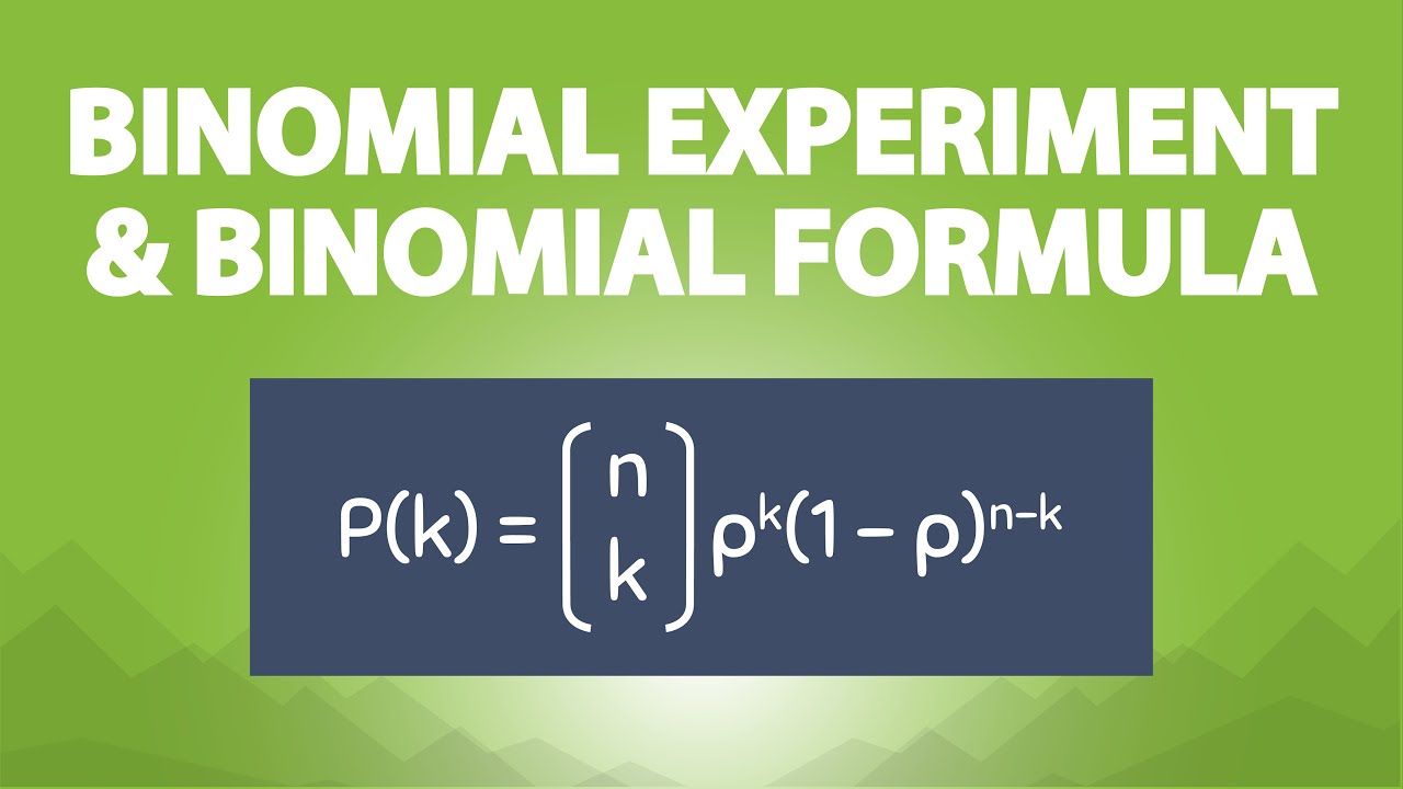
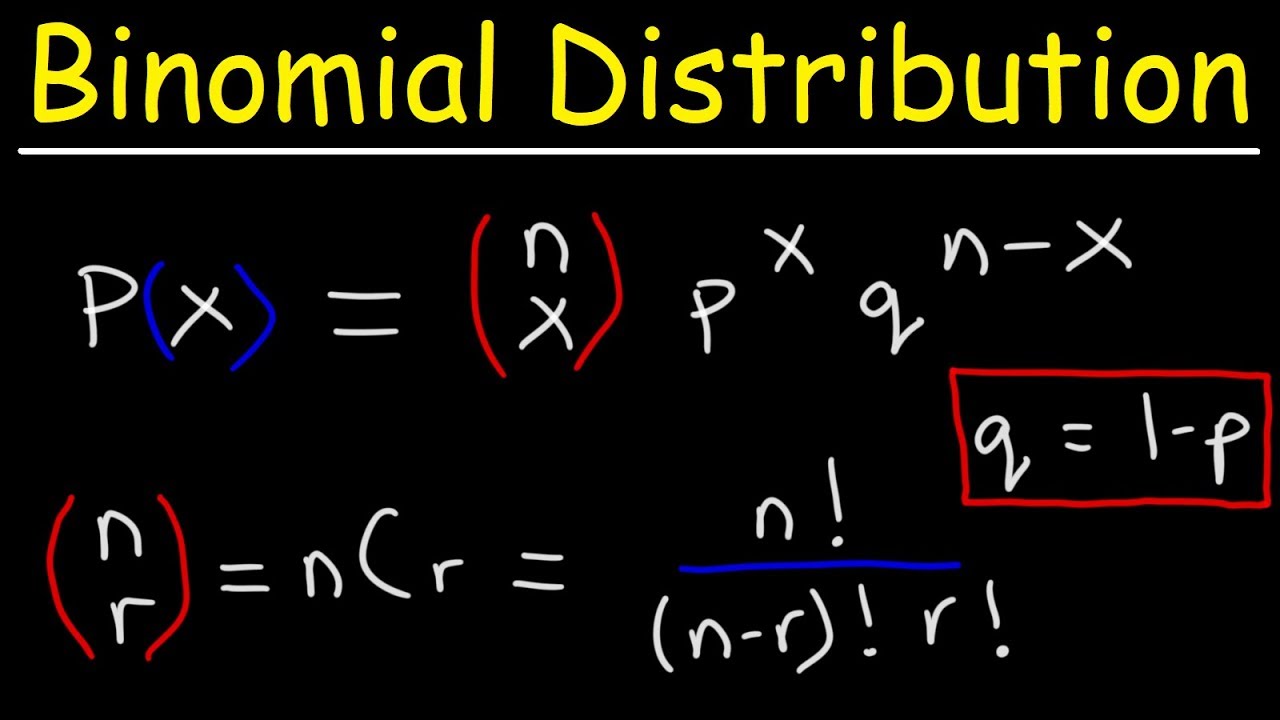
What is the binomial probability formula used to calculate the probability of getting exactly x successes in n trials?
-The binomial probability formula is used to calculate the probability of getting exactly x successes in n trials and is given by: P(x) = (n choose x) * (p^x) * (q^(n-x)), where 'n choose x' is the binomial coefficient, p is the probability of success, and q is the probability of failure.
How can you find the probability of at least 11 Mexican-American jurors out of 12 using the binomial distribution?
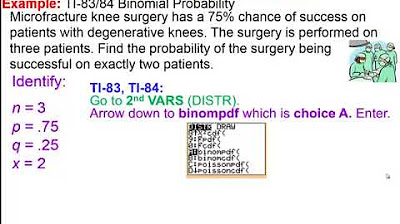
-To find the probability of at least 11 Mexican-American jurors out of 12, you would calculate the sum of the probabilities of getting exactly 11 and exactly 12 Mexican-American jurors using the binomial probability formula or a calculator with a binomial PDF function.
What is the mean, variance, and standard deviation of a binomial distribution, and how are they calculated?
-The mean (μ) of a binomial distribution is calculated as n * p, the variance is calculated as n * p * q, and the standard deviation is the square root of the variance, which is √(n * p * q), where n is the number of trials, p is the probability of success, and q is the probability of failure.
How can you determine if it is unusual to have only three Mexican-American jurors on a jury, given the population is 80% Mexican-American?
-To determine if it is unusual to have only three Mexican-American jurors, you can calculate the mean and standard deviation of the binomial distribution for the number of Mexican-American jurors. Then, use the rule of thumb that any result more than two standard deviations away from the mean is unusual. In this case, the minimum usual value would be calculated as mean - 2 * standard deviation.
Outlines
📚 Introduction to Binomial Probability Distribution
The video script begins with an introduction to the second half of chapter five, focusing on the binomial probability distribution. This discrete probability distribution is used to model situations with two possible outcomes, such as yes/no, heads/tails, or success/failure. The script explains the conditions for binomial distribution, including a fixed number of trials (n), independent events, and two possible outcomes with constant probabilities of success (p) and failure (q). An example of flipping a fair coin ten times is used to illustrate these concepts, with a detailed explanation of how to set up and interpret the binomial distribution for this scenario.
🧬 Applying Binomial Distribution to Genetics and Jurors
The script continues with examples of applying the binomial distribution to genetics and jury selection. It discusses how the number of children with type O blood from a pair of parents can be modeled using a binomial variable, given the probability of having type O blood is 0.25. Another example involves selecting jurors from a population where 80% are Mexican-American, using the binomial distribution to calculate the probability of having a certain number of Mexican-American jurors in a group of 12. The script emphasizes checking the conditions for binomial distribution and calculating probabilities using the binomial formula or calculator functions.
🔢 Using Calculator Functions for Binomial Probability
The script provides a step-by-step guide on how to use calculator functions to find binomial probabilities. It explains the process of using the binomial PDF (probability density function) for exact probabilities and the binomial CDF (cumulative distribution function) for cumulative probabilities. The script demonstrates how to calculate the probability of having exactly seven Mexican-American jurors out of 12 and the probability of having at least 11. It also discusses an alternative method using the CDF to find the probability of a range of outcomes more efficiently.
📉 Calculating Mean, Variance, and Standard Deviation
The script shifts focus to explaining how to calculate the mean, variance, and standard deviation for binomial distributions. It presents simplified formulas for these calculations, which are derived from the general formulas for discrete probability distributions. The script uses the example of the jury problem to illustrate how to find the mean and standard deviation, providing the expected number of Mexican-American jurors and the measure of dispersion around this mean. It emphasizes the importance of using a calculator for these calculations to save time and avoid errors.
📊 Comparing Calculation Methods for Mean and Standard Deviation
This section of the script compares the simplified binomial formulas for calculating the mean and standard deviation with the more traditional method involving summing up individual probabilities. The script shows the calculations for both methods, highlighting the discrepancies that may arise due to rounding errors or early rounding off. It demonstrates that while the simplified method is faster and more efficient, the traditional method can provide a more precise result if done carefully.
🏷️ Determining Usual Values and Unusual Outcomes
The script concludes with a discussion on determining usual values and identifying unusual outcomes in binomial distributions. Using the jury example, it calculates the minimum and maximum usual values based on the mean and standard deviation, showing that having only three Mexican-American jurors would be considered unusual given the 80% population proportion. The script also presents a new scenario involving the proportion of overweight Americans in a town, calculating the mean and standard deviation for the number of overweight people in a town of 40,000 residents.
📘 Summary of Binomial Distribution Concepts
In the final paragraph, the script summarizes the key concepts covered in the video, including the conditions for binomial distribution, the use of calculator functions for probability calculations, and the simplified formulas for mean, variance, and standard deviation. It encourages students to attend class with questions and reiterates the importance of understanding these concepts for solving binomial distribution problems efficiently.
Mindmap
Keywords
💡Binomial Probability Distribution
💡Fixed Number of Trials (n)
💡Independent Events
💡Success and Failure
💡Probability of Success (p)
💡Complement (q)
💡Binomial Random Variable (x)
💡Binomial Coefficient
💡Binomial PDF (Probability Density Function)
💡Binomial CDF (Cumulative Distribution Function)
💡Mean, Variance, and Standard Deviation
Highlights
Introduction to the second half of chapter five focusing on the binomial probability distribution.
Explanation of binomial distribution as a discrete probability distribution for events with two possible outcomes.
Conditions for binomial distribution: fixed number of trials, independent events, and two possible outcomes labeled as success and failure.
The probability of success (p) and failure (q) in binomial distribution, with q being one minus p.
Example of binomial distribution using ten coin flips with a fair coin.
Illustration of how to set up a binomial distribution problem with a fixed number of trials, independent outcomes, and defined success/failure probabilities.
Use of binomial distribution in genetics to determine the probability of children having type O blood from parents with a 0.25 probability.
Application of binomial distribution in a juror selection scenario with a large, independent population.
Two methods for finding binomial probabilities: using the binomial probability formula and calculator functions.
Demonstration of using a calculator's binomial PDF function to find the probability of exactly x successes.
Explanation of binomial coefficient and its role in the binomial probability formula.
Alternative method using binomial CDF function on a calculator to find cumulative probabilities.
Calculation of mean, variance, and standard deviation for binomial distributions using shortcuts.
Example of finding the mean and standard deviation for the number of Mexican-American jurors in a 12-person jury.
Discussion on determining unusual values using the mean and standard deviation in binomial distribution.
Application of binomial distribution to a real-world scenario of overweight Americans in a town of 40,000 people.
Advantages of using binomial distribution formulas for mean and standard deviation over general distribution calculations.
Conclusion and invitation for students to bring questions to the next class.
Transcripts
Browse More Related Video
Elementary Statistics - Chapter 5 Binomial Distributions Part 2
The Binomial Experiment and the Binomial Formula (6.5)

Binomial Distribution EXPLAINED in UNDER 15 MINUTES!

Bernoulli, Binomial and Poisson Random Variables
5.2.1 Binomial Probability Distributions - Is this procedure described by a binomial distribution?
Finding The Probability of a Binomial Distribution Plus Mean & Standard Deviation
5.0 / 5 (0 votes)
Thanks for rating: