Checking assumptions of the linear model
TLDRThe video script discusses the assumptions of linear models and methods to check them, focusing on the examination of residuals. The key assumptions covered include the absence of measurement error in independent variables, independence of errors, normal distribution of errors, constant variance, and linearity of the relationship between X and Y. The script emphasizes the use of residual plots, such as histograms, normal quantile plots, residual vs. fitted values, scale-location plots, and leverage plots, to visually assess these assumptions. It highlights the importance of identifying and addressing deviations, particularly extreme points, to ensure the validity and reliability of the model.
Takeaways
- 🔍 The assumptions of a linear model include that independent variables are measured without error, errors are independent, residuals are normally distributed with constant variance, and the relationship between X and Y is linear.
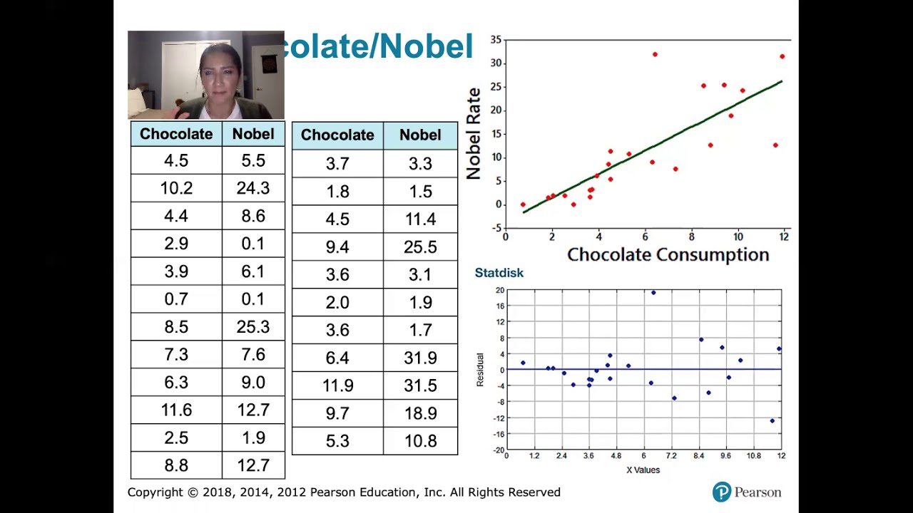
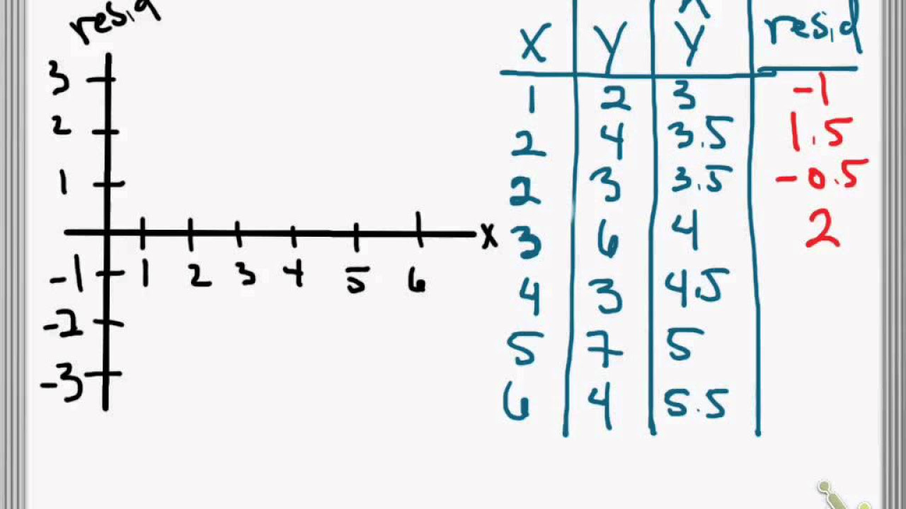
- 📊 To check these assumptions, one can use graphical methods such as examining plots of residuals, which are the deviations between the predicted and actual values.
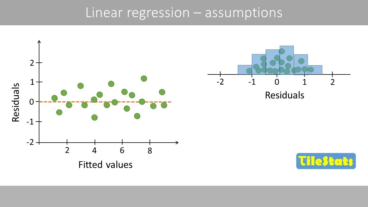
- 📈 A histogram of residuals can provide a visual test for normal distribution, showing if residuals are symmetrically distributed around zero.
- 📝 A quantile-quantile (Q-Q) plot can help verify if residuals follow a normal distribution by comparing sample quantiles to theoretical quantiles.
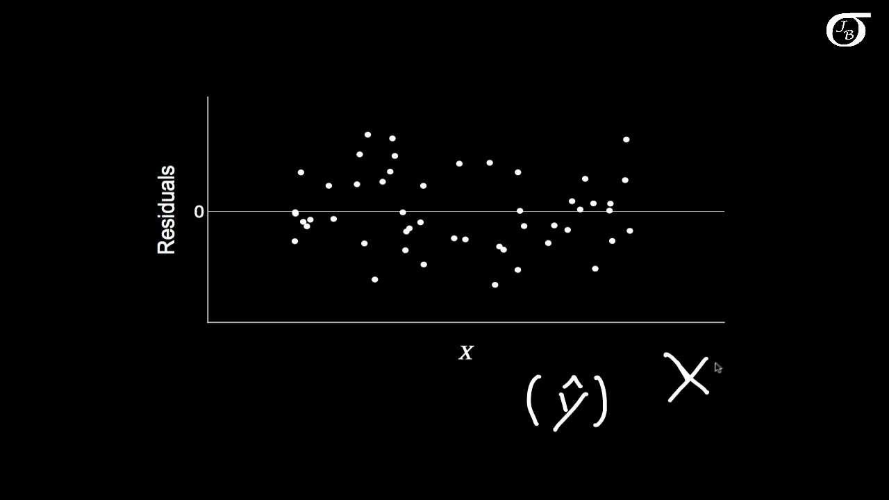
- 📊 Residuals vs. fitted values plot can reveal if there's an even scatter of points around the horizontal line representing the predicted mean value, indicating no systematic error.
- 📈 The scale-location plot, which rescales the residuals by their estimated error, can detect departures from the assumption of constant variance.
- 🔍 Large outliers in the scale-location plot can indicate points that do not fit the model well and may need further investigation.
- 📊 A plot of standardized residuals against leverage can identify influential points that have a significant impact on the model fit.
- 🔗 High leverage points with large residuals suggest that the model fit is poor and these points may influence the outcome significantly.
- 🛠️ Removing extreme points can lead to changes in the fitted model, potentially improving the fit and flattening the fitted line.
- 📈 After removing influential points, the Q-Q plot and residual vs. independent variable plot can show improvements, indicating a better fit to the data.
Q & A
What are the assumptions of a linear model?
-The assumptions of a linear model include that the independent variables are measured without error, the errors are independent, the errors are normally distributed, have a constant variance, and the relationship between the X variable and the average Y is linear.
How can we check if the independent variables are measured without error?
-In practice, it is almost always violated to assume that independent variables are measured without error. This violation is often ignored as it is very common in real-world scenarios.
What is the role of residual plots in assessing the assumptions of a linear model?
-Residual plots are used to graphically examine the deviations between the average value of Y predicted by the model and a particular observation. They help in checking if the assumptions of the linear model are met, particularly the normality, constant variance, and linearity of the relationship between X and Y.
How can a histogram of residuals help in assessing normality?
-A histogram of residuals can visually test whether the residuals are normally distributed. If there are more residuals close to zero and it is roughly symmetrical, it suggests that the residuals could be normally distributed, although it is not easy to judge with certainty.
What is a quantile-quantile (Q-Q) plot and how does it help in assessing the normality of residuals?
-A quantile-quantile plot is a graphical tool where the theoretical quantiles are plotted on the x-axis and the sample quantiles for the data points are plotted on the y-axis. If the data follows a normal distribution, the points should fall along a straight line. Deviations from this line, especially in the tails, indicate that the residuals may not be normally distributed.
What does a plot of residuals versus fitted values show?
-A plot of residuals versus fitted values shows the residual (error) on the y-axis and the predicted mean value for each observation on the x-axis. If the assumptions are correct, the points should be scattered evenly above and below a horizontal line, indicating no systematic pattern.
What is the significance of a scale-location plot?
-A scale-location plot is similar to a residuals versus fitted values plot, but the y-axis has been rescaled by taking the absolute value of the residuals and then scaling them by the estimated error in the model, followed by taking the square root. This plot helps in assessing whether the variance is constant, as a flat line without any trend indicates that the assumption of constant variance is met.
How can we identify influential points in a linear model?
-Influential points can be identified by examining a plot with standardized residuals on the y-axis and leverage on the x-axis. High leverage points with large residuals indicate that the model fit is significantly impacted by these points, and they may need to be considered for removal.
What is the impact of removing extreme points from a linear model?
-Removing extreme points can change the fitted line of the model. For example, after removing point 141 and three other extreme points from the dataset, the fitted line becomes flatter, indicating a change in the slope and suggesting that the model fit was previously influenced by those points.
What is the purpose of a Cook's distance plot?
-A Cook's distance plot helps identify points that have a large influence on the model. It measures the impact of each observation and points that are far out in the corners with large Cook's distances may be considered for removal as they could be influencing the model fit.
How does the removal of influential points affect the quantile-quantile plot?
-The removal of influential points can significantly improve the quantile-quantile plot. After removing point 141 and three other extreme points, the plot shows a much straighter line, indicating a better fit to the normal distribution assumption.
Outlines
📊 Linear Model Assumptions and Residual Analysis
This paragraph discusses the assumptions underlying a linear model and the importance of checking whether these assumptions are met. The key assumptions include the absence of measurement error in independent variables, independence of errors, normal distribution of errors, constant variance, and linearity of the relationship between the X variable and the average Y. The speaker emphasizes the common practice of ignoring minor violations of these assumptions in real-world scenarios. The primary method for examining these assumptions is through graphical analysis of residuals, which are the deviations between the predicted Y values and the actual observations. The speaker describes the use of histograms, quantile-quantile plots, and residual versus fitted value plots to assess the normality, variance, and linearity of the data. The paragraph highlights the significance of these diagnostic plots in identifying potential issues with the model, such as extreme values or non-linear relationships.
📈 Advanced Residual Analysis and Outlier Detection
The second paragraph delves deeper into the analysis of residuals and the detection of outliers. It introduces additional diagnostic plots such as the scale-location plot and leverage plot. The scale-location plot, which uses the absolute value of residuals and scales them by the estimated error, helps detect departures from the assumption of constant variance. The leverage plot, on the other hand, measures the influence of individual observations on the model fit, highlighting points with high leverage and large residuals that may indicate a poor fit and significant impact on the model. The speaker also discusses the concept of Cook's distance, another measure of influence, and the importance of examining points with large Cook's distance. The paragraph concludes with an example of how removing extreme points can alter the fitted model, leading to a flatter and potentially more accurate linear fit, as evidenced by improvements in the quantile-quantile plot and the residual versus independent variable plot.
Mindmap
Keywords
💡Assumptions
💡Residuals
💡Quantile-Quantile Plot
💡Normal Distribution
💡Constant Variance
💡Linear Relationship
💡Fitted Values
💡Leverage
💡Cook's Distance
💡Scale-Location Plot
💡Influential Points
Highlights
Assumptions of the linear model are crucial for its validity and need to be checked.
Independent variables on the x-axis are assumed to be measured without error, which is often violated in practice.
Errors are assumed to be independent, meaning one observation's error does not inform about the next observation's error.
Residuals, the deviations between the predicted and actual values, are assumed to be normally distributed.
The variance of residuals is assumed to be constant across all levels of the independent variable.
The relationship between the X variable and the average Y is assumed to be linear.
Graphical examination of plots is a common method to check the assumptions of the linear model.
Histograms of residuals can provide a visual test for normal distribution.
Quantile-quantile (Q-Q) plots are used to check if residuals follow a normal distribution.
Residuals versus fitted values plot can reveal if the assumptions hold true.
Scale-location plot can detect departures from the assumption of constant variance.
Systematic deviation in residuals may indicate a nonlinear relationship between X and Y.
Leverage plot helps identify observations that have a large impact on the model fit.
High leverage points with large residuals suggest a poor fit by the model and significant influence on the result.
Cook's distance is another measure to assess the influence of individual observations on the model fit.
Removing extreme points can improve the fit and assumptions of the linear model.
After removing influential points, the Q-Q plot and residual versus independent variable plot can show significant improvement.
Transcripts
Browse More Related Video
10.2.6 Regression - Residual Plots and Their Interpretation
Simple Linear Regression: Checking Assumptions with Residual Plots
Assumptions in Linear Regression - explained | residual analysis

Regression assumptions explained!
Residuals and Residual Plots

Checking Linear Regression Assumptions in R | R Tutorial 5.2 | MarinStatsLectures
5.0 / 5 (0 votes)
Thanks for rating: