Assumptions in Linear Regression - explained | residual analysis
TLDRThis video delves into the assumptions behind linear regression analysis, focusing on five key aspects: linearity, homoscedasticity, normality, independence, and absence of multicollinearity. It explains how to create and interpret residual plots to check these assumptions, highlighting the importance of each for the validity of the regression model. The video also discusses methods to address violations, such as data transformation, outlier detection using Cook's distance, and techniques like weighted least squares regression and principal component regression.
Takeaways
- 📈 Linear Regression Assumptions: The video discusses the assumptions necessary for linear regression analysis, emphasizing the importance of checking these assumptions for accurate modeling and interpretation.
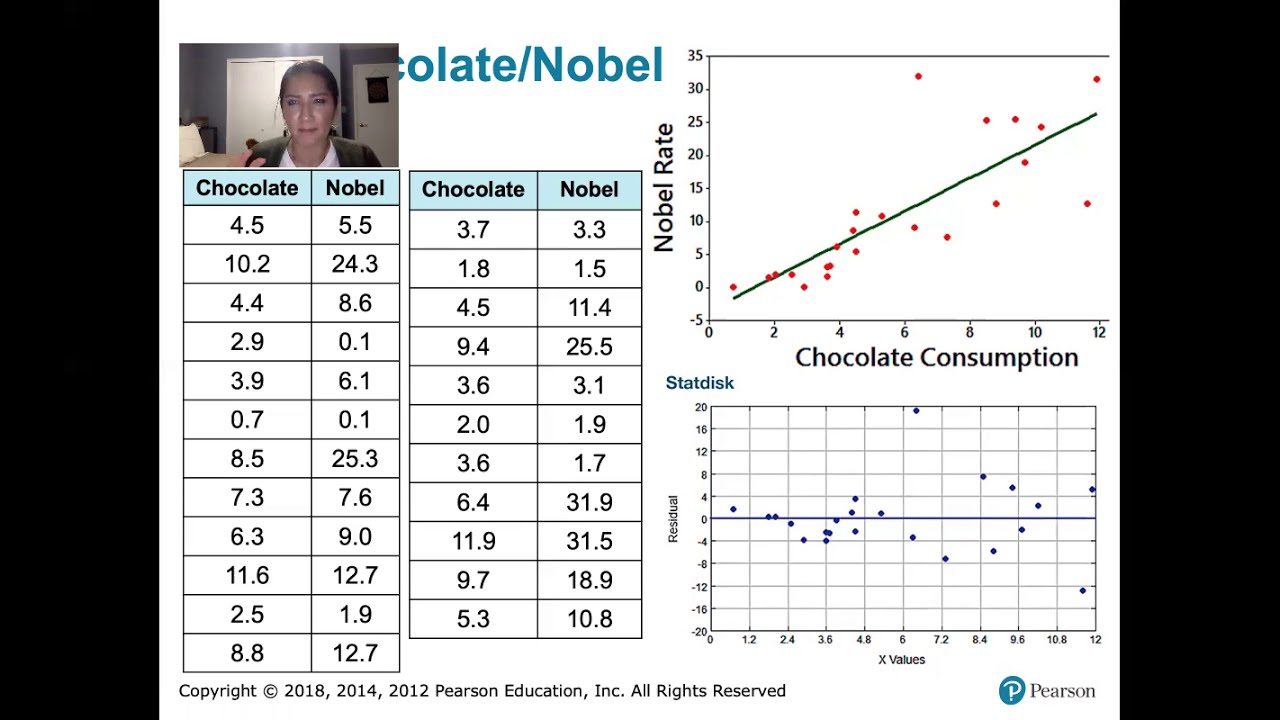
- 📊 Residual Analysis: The process of analyzing residuals is crucial for validating the assumptions of linear regression. It involves comparing the observed values to the estimated or predicted values derived from the regression model.
- 🤔 Understanding Residuals: Residuals are the differences between the actual data points (Absurd values) and the estimated values (predicted by the regression line). They are used to evaluate the fit of the regression model to the data.
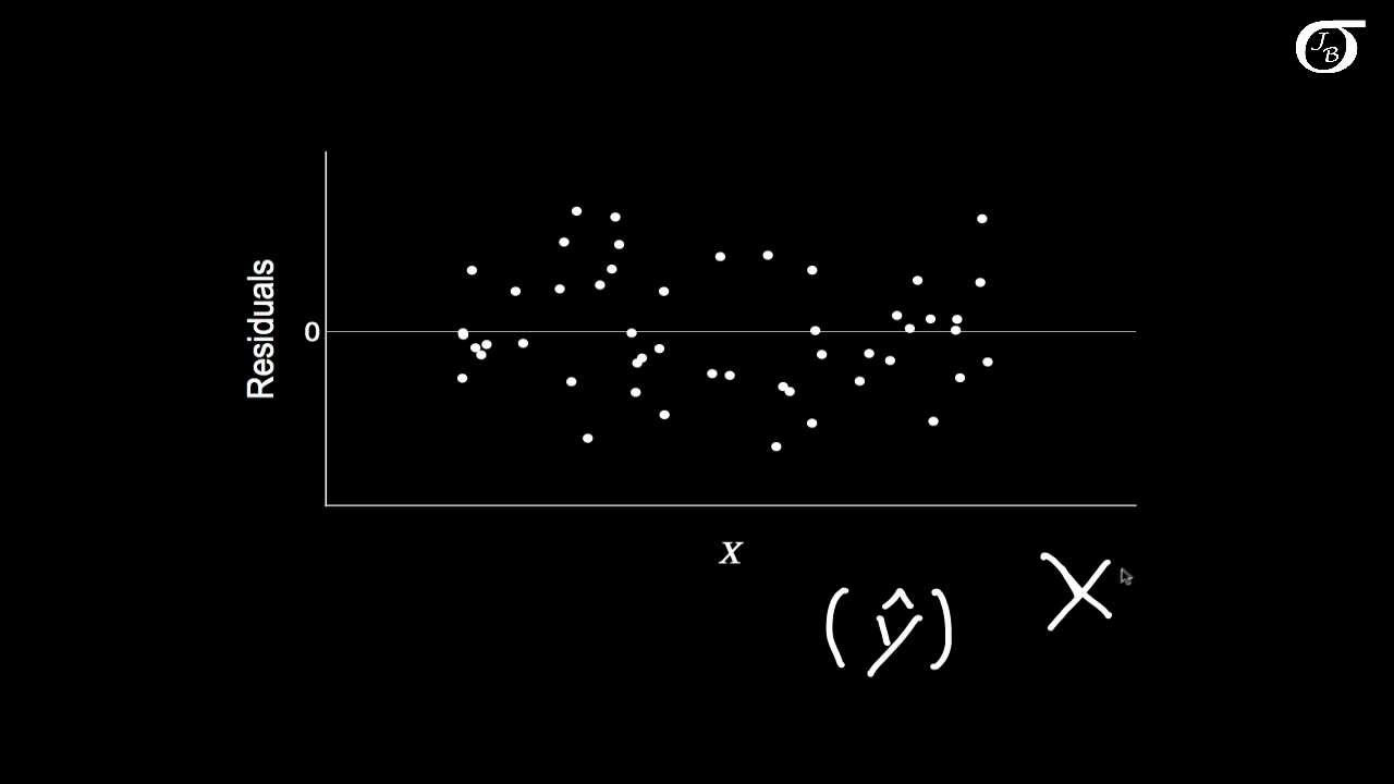
- 📉 Creating a Residual Plot: A residual plot is created by plotting the residuals against the X values or the estimated Y values (fitted values). This helps in identifying patterns and potential issues with the regression model assumptions.
- 🔍 Assumption of Linearity: The first assumption for linear regression is that there should be a linear relationship between the independent variable (X) and the dependent variable (Y), which should be evident when data points are spread around a straight line in the residual plot.
- 📏 Homoscedasticity: The assumption of homoscedasticity requires that the spread of the residuals (variance) should be constant along the regression line. Violation of this assumption can lead to increased risk of Type 1 error in the model.
- 🔢 Normality: The residuals should be normally distributed around the regression line. This can be assessed using histograms and quantile-quantile (QQ) plots. Non-normality may indicate the need for data transformation or the inclusion of additional variables.
- 🚫 Outliers and Influence: Outliers can significantly influence the regression line and should be identified and addressed. Cook's distance is a method used to measure the influence of individual data points on the regression model.
- 🔄 Independence: The assumption of independence states that the residuals should not show any pattern over time or order of data collection. Durbin-Watson's test can be used to check for autocorrelation in the residuals.
- 🔍 Collinearity: The final assumption checks for collinearity among independent variables. High correlation between predictors can lead to unreliable parameter estimates and inflated variances. Variance Inflation Factor (VIF) is used to detect collinearity.
- 🛠 Addressing Violations: If any of the assumptions are violated, appropriate statistical techniques or transformations should be applied to address the issues, ensuring the validity and reliability of the linear regression analysis.
Q & A
What is the primary purpose of residual analysis in linear regression?
-The primary purpose of residual analysis in linear regression is to evaluate the assumptions of the model by examining the residuals, which are the differences between the actual data points and the estimated values predicted by the regression line.
How is a residual plot created?
-A residual plot is created by plotting the residuals on one axis (usually the y-axis) against the estimated values or fitted values on the other axis (usually the x-axis). This helps in visualizing the pattern of residuals and assessing the validity of the regression model's assumptions.
What does the equation of a regression line represent?
-The equation of a regression line represents the best-fit line through a set of data points, which can be used to predict the response variable (dependent variable) based on the independent variable(s). It is derived from the data using the method of least squares.
What is the significance of the estimated or fitted values in linear regression?
-The estimated or fitted values are the predicted values of the response variable obtained from the regression line equation for each level of the independent variable(s). They are crucial for calculating residuals and assessing the accuracy and fit of the regression model.
What does the assumption of linearity imply in the context of linear regression?
-The assumption of linearity implies that there is a straight-line relationship between the independent variable(s) and the dependent variable. This means that the data points should be evenly spread around a straight line, and the corresponding residual plot should show residuals evenly distributed along the reference line.
How can you identify a violation of the homoscedasticity assumption?
-A violation of the homoscedasticity assumption can be identified by observing the residual plot, where the spread of residuals (the distance from the data points to the reference line) should be constant along the regression line. If the spread increases or decreases along the line, it indicates a violation of homoscedasticity.
What is the impact of unequal variance on the regression model?
-Unequal variance increases the risk of a Type 1 error, as the p-values associated with the estimated parameters in the regression model become smaller compared to the case with equal variance. This can lead to incorrect conclusions about the significance of the model's predictors.
What are some methods to address the issue of unequal variance in the data?
-Methods to address unequal variance include using a Poisson regression model (for count data), transforming the data, computing robust standard errors, or using weighted least squares regression. These methods help to reduce the risk of committing a Type 1 error and improve the model's accuracy.
How can you determine if the normality assumption is met in a linear regression model?
-To determine if the normality assumption is met, you can create a histogram of the residuals and imagine a normal distribution curve. Additionally, a quantile-quantile (Q-Q) plot can be used, where the data points should be distributed along a straight reference line if the residuals are normally distributed.
What are some consequences of violating the normality assumption in linear regression?
-Violating the normality assumption can lead to biased estimates and inflated standard errors, which in turn can affect the reliability of the model's predictions and the interpretation of the regression coefficients. It may also impact the validity of hypothesis tests performed on the model parameters.
How can you detect and deal with outliers in a linear regression model?
-Outliers can be detected using Cook's distance, which measures the influence of a data point on the regression line. A data point with a Cook's distance greater than a critical value (typically based on the sample size and number of explanatory variables) may be considered an outlier. To deal with outliers, one can consider removing them, correcting measurement errors, or using robust methods that are less sensitive to outliers.
What is the assumption of independence in linear regression, and why is it important?
-The assumption of independence states that the data points should not be correlated with each other in terms of their order of collection. This is important because if there is a pattern in the residuals over time, it indicates that the measurements are dependent on the order they were collected, which can lead to biased estimates and incorrect conclusions.
How can you test for the assumption of independence in a linear regression model?
-The assumption of independence can be tested using the Durbin-Watson test statistic, which measures the degree of autocorrelation in the residuals. A value close to 2 indicates that the residuals are uncorrelated, while values significantly less than 2 or greater than 3 suggest a problem with autocorrelation.
What is collinearity in the context of linear regression, and how can it be identified?
-Collinearity occurs when two or more independent variables in the model are highly correlated with each other. This can be identified by computing the variance inflation factor (VIF) for each variable. A VIF greater than 5 or especially greater than 10 indicates a problem of collinearity.
What are some strategies to address collinearity in a linear regression model?
-To address collinearity, one can consider deleting one of the highly correlated variables, combining the correlated variables into a single predictor (e.g., calculating the body mass index from body weight and height), or using statistical methods like principal component regression or partial least squares regression that can handle multicollinearity.
Outlines
📊 Introduction to Residual Analysis and Assumptions in Linear Regression
This paragraph introduces the concept of residual analysis and its importance in verifying the assumptions of linear regression. It explains that residuals are the differences between the actual data points and the estimated values predicted by the regression line. The paragraph also describes how to create a residual plot and emphasizes the necessity of fulfilling certain assumptions for the validity of the linear regression model. These assumptions include linearity, homoscedasticity, normality, independence, and absence of collinearity. The discussion begins with the assumption of linearity, highlighting the need for data points to be distributed around a straight line and how a residual plot can reveal violations of this assumption.
📈 Violations of Homoscedasticity and Its Implications
The second paragraph delves into the assumption of homoscedasticity, which requires a constant spread of residuals along the regression line. It explains how violations of this assumption, such as increasing variance along the regression line, can affect the residual plot and lead to smaller P values, increasing the risk of Type 1 error. The paragraph suggests solutions like using a Poisson regression model for count data or transforming the data to address unequal variance. It also discusses the use of robust standard errors and weighted least squares regression as alternatives to handle violations of homoscedasticity.
📊 Identifying and Dealing with Non-Normality in Residuals
This paragraph addresses the assumption of normality, which posits that data points should be normally distributed around the regression line. It describes how to analyze the distribution of residuals using histograms and quantile-quantile (QQ) plots. The paragraph also discusses the implications of non-normality, such as biased estimates and the potential influence of outliers. It presents methods for identifying outliers, like Cook's distance, and suggests remedies such as data transformation or removal of outliers. The importance of including more explanatory variables to achieve normal distribution of residuals is highlighted, as well as the potential issues caused by missing variables or outliers.
🔍 Detecting and Ensuring Independence of Residuals
The fourth paragraph focuses on the assumption of independence, which requires that residuals should not show any pattern over time. It discusses how the order of data collection can affect the residuals and how to identify patterns using the Durbin-Watson test statistic. The paragraph suggests that a value close to 2 indicates uncorrelated residuals, while values less than 1 or greater than 3 suggest a violation of the independence assumption. Solutions to address this issue include adjusting the data collection method or using statistical techniques designed to handle autocorrelation, such as time series analysis or generalized estimating equations.
🔧 Addressing Collinearity in Multiple Regression Models
The final paragraph discusses the assumption of no collinearity, which is crucial when interpreting the effects of multiple explanatory variables in a model. It explains how strong correlations between independent variables can lead to problematic estimates and inflated P-values. The paragraph describes methods to identify collinearity, such as calculating the variance inflation factor (VIF), and suggests solutions like deleting or combining correlated variables, creating new variables that capture the essence of the correlated ones, or employing statistical methods like principal component regression or partial least squares regression to mitigate the effects of collinearity.
Mindmap
Keywords
💡Residual Analysis
💡Linear Regression
💡Homoscedasticity
💡Normality
💡Independence
💡Collinearity
💡Cook's Distance
💡Variance Inflation Factor (VIF)
💡Durbin-Watson Test
💡Residual Plot
💡Transforming Data
Highlights
The video discusses residual analysis and assumptions in linear regression, providing a comprehensive understanding of how to validate and interpret regression models.
Five key assumptions in linear regression are covered, offering insights into how to check if a model fulfills these assumptions for accurate analysis.
A step-by-step guide on creating a residual plot is provided, which is essential for visualizing the relationship between the regression line and data points.
The concept of estimated or predicted values is introduced, explaining how they are calculated and their significance in regression analysis.
The importance of linearity in the relationship between the independent and dependent variables is emphasized, with examples of how to identify and address violations of this assumption.
Homoscedasticity is explained as the assumption that the spread of residuals should be constant along the regression line, with illustrations of its violation and potential solutions.
The normality assumption is discussed, highlighting the need for residuals to be normally distributed and methods to assess and address deviations from this assumption.
Independence of residuals is crucial, and the video explains how to detect and handle situations where residuals show patterns over time or are influenced by the order of data collection.
Collinearity among independent variables is identified as a potential issue, with the video providing strategies for detecting and mitigating its impact on regression analysis.
The video demonstrates the use of Cook's distance to identify outliers and the importance of addressing these to ensure the robustness of regression models.
The Durbin-Watson test is introduced as a method to check for the assumption of independence in residuals, with guidance on interpreting the test statistic.
The concept of variance inflation factor is explained, offering a quantitative measure for detecting collinearity among independent variables.
Strategies to deal with collinearity, such as variable deletion, combination, or the use of advanced regression techniques, are suggested to improve model interpretability and accuracy.
The video concludes with a summary of the assumptions behind linear regression and their practical implications for data analysis and model interpretation.
Throughout the video, the presenter uses clear examples and visual aids to illustrate complex concepts, making the material accessible to a wide audience.
The video emphasizes the importance of validating assumptions before drawing conclusions from regression analysis, ensuring the reliability of the results.
Transcripts
Browse More Related Video

Checking Linear Regression Assumptions in R | R Tutorial 5.2 | MarinStatsLectures

Regression assumptions explained!

What is Multicollinearity? Extensive video + simulation!
10.2.6 Regression - Residual Plots and Their Interpretation
Simple Linear Regression: Checking Assumptions with Residual Plots

Regression diagnostics and analysis workflow
5.0 / 5 (0 votes)
Thanks for rating: