Regression assumptions explained!
TLDRThe video script by Justin Zeltser from Zed, Statistics Calm delves into the critical assumptions underlying regression analysis. It discusses six key assumptions, including linearity, constant error variance (homoscedasticity), independent error terms, normal errors, no multicollinearity, and exogeneity (avoiding omitted variable bias). The video emphasizes the importance of these assumptions for reliable coefficients and standard errors, and provides methods for detecting and remedying violations of these assumptions, ensuring accurate and valid regression models.
Takeaways
- 📊 Regression analysis relies on several key assumptions, including linearity, constant error variance (homoscedasticity), independent error terms, normal errors, no multicollinearity, and exogeneity.
- 🔍 The linearity assumption requires the relationship between the dependent and independent variables to be linear, which can be achieved through transformations like including squared terms if necessary.
- 🎯 Violation of the constant error variance assumption leads to heteroscedasticity, which affects the reliability of standard errors and hypothesis testing.
- 🔄 The independence of error terms assumption ensures that each error is uncorrelated with the others; autocorrelation, or serial correlation, indicates a violation and can be detected using tests like Durbin-Watson.
- 📈 Normal errors assumption states that the error terms should be normally distributed, which is important for the validity of statistical tests; large sample sizes can mitigate issues with normality violations.
- 🔗 Multicollinearity occurs when independent variables are highly correlated with each other, leading to unreliable coefficients and standard errors; it can be detected using correlation analysis and variance inflation factor.
- 🔒 Exogeneity ensures that the independent variables are not related to the error term; omitted variable bias is a form of endogeneity where a relevant variable is not included in the model, affecting the causative interpretation of coefficients.
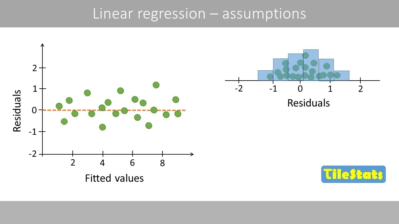
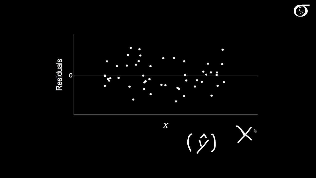
- 🛠️ Residual plots are a useful diagnostic tool for identifying violations of regression assumptions, such as patterns indicating non-linearity or heteroscedasticity.
- 📝 Correct functional form is crucial for reliable regression analysis; an incorrect form can lead to both coefficients and standard errors being unreliable, rendering the regression useless.
- 📊 Transformations like logging or using different variable forms can often resolve issues with heteroscedasticity and multicollinearity.
- 🎓 Understanding and testing for these regression assumptions is vital to ensure the validity of the regression analysis and to avoid drawing incorrect conclusions from the data.
Q & A
What are the six assumptions discussed in the video related to regression analysis?
-The six assumptions discussed are linearity, constant error variance (homoscedasticity), independent error terms, normal errors, no multicollinearity, and exogeneity (no omitted variable bias).
How does the assumption of linearity relate to the functional form in a regression model?
-Linearity assumes that the relationship between the dependent variable and the independent variables is linear. This means the model is additive and can include transformations like X^2 or log(X) without violating the assumption, as long as the relationship can be expressed in a linear equation.
What is the implication of violating the constant error variance assumption?
-Violating the constant error variance assumption, also known as heteroscedasticity, means that the spread or variance of the error terms changes as the independent variable(s) change. This can lead to unreliable standard errors and affects the validity of hypothesis tests based on these errors.
How can we detect the presence of heteroscedasticity in a regression model?
-Heteroscedasticity can be detected by examining a residual plot, which should show a consistent spread of residuals across different levels of the independent variable(s). If the spread increases or decreases with the independent variable(s), heteroscedasticity may be present. Formal tests like the Goldfeld-Quandt test or the Breusch-Pagan test can also be used.
What is autocorrelation and why is it a concern in regression analysis?
-Autocorrelation, or serial correlation, occurs when there is a correlation between successive error terms in a time series regression model. This violates the assumption of independent error terms and can lead to unreliable standard errors, affecting the validity of hypothesis tests and the confidence in the model's coefficients.
How can we address the issue of autocorrelation in a regression model?
-To address autocorrelation, one can include additional variables that may account for the observed pattern, such as lagged variables or other economic indicators. Alternatively, using generalized least squares or differencing the data to create a new variable that models the change over time can help. These methods help to remove the autocorrelation from the error terms.
What does the assumption of normal errors mean in the context of regression?
-The assumption of normal errors means that the distribution of the error terms should be normally distributed, with most of the data centered around zero and fewer observations as we move further away from zero. This assumption is important for the validity of hypothesis tests and confidence intervals in the model.
How can we assess whether the error terms in a regression model are normally distributed?
-Normality of error terms can be assessed by examining a histogram or a QQ plot of the residuals. The histogram should show a bell-shaped curve, and the QQ plot should display a straight line if the residuals are normally distributed. Deviations from these patterns indicate non-normality.
What is multicollinearity and how does it affect a regression model?
-Multicollinearity occurs when the independent variables in a regression model are highly correlated with each other. This can lead to unreliable and unstable estimates of the regression coefficients and standard errors, making it difficult to interpret the individual effects of the variables on the dependent variable.
What are some ways to address multicollinearity in a regression model?
-To address multicollinearity, one can remove or combine highly correlated variables, add variables that provide additional information without being collinear, or use techniques like ridge regression or principal component analysis to reduce the correlation between variables.
What is the issue with omitted variable bias in a regression model?
-Omitted variable bias occurs when a relevant variable that affects the dependent variable is not included in the model. This can lead to incorrect estimates of the coefficients for the included variables, as the omitted variable's effect is confounded with the effects of the included variables.
How can we attempt to correct for omitted variable bias in a regression model?
-Correcting for omitted variable bias can be challenging as it requires identifying and including the omitted variables. In some cases, using instrumental variables or conducting randomized controlled trials can help isolate the effect of the included variables. However, this is often not feasible, and researchers must rely on their understanding of the subject matter to make informed decisions about which variables to include.
Outlines
📊 Introduction to Regression Assumptions
This paragraph introduces the topic of regression assumptions, highlighting the importance of understanding the assumptions that underpin regression analysis. It mentions that there are varying numbers of assumptions discussed in different sources, but the video will focus on six key assumptions. The speaker, Justin Zeltser, emphasizes his approach of explaining concepts intuitively without unnecessary formulas, aiming to make the material highly intelligible. The paragraph also briefly describes the graphical representation of regression, including the scatterplot of observations and the line of best fit.
🔍 Linearity Assumption and Its Violation
The second paragraph delves into the first assumption of linearity, explaining that it means the relationship between the variables should be additive and linear. It clarifies that including transformations like X squared or log X in the regression equation does not violate the linearity assumption. The speaker uses the example of assessing lung function based on age and discusses how an incorrect functional form can lead to unreliable coefficients and standard errors. The paragraph also introduces residual plots as a tool for detecting issues with the functional form and mentions the use of likelihood ratio tests for comparing models.
📈 Constant Error Variance (Homoscedasticity)
This paragraph discusses the assumption of constant error variance, also known as homoscedasticity, which implies that the variance of the error terms should be constant across different levels of the independent variable. The speaker provides an example of household expenditure as a function of income and explains how heteroscedasticity, the violation of this assumption, can occur. The paragraph describes the impact of heteroscedasticity on the reliability of standard errors and hypothesis testing. It also mentions methods for detecting heteroscedasticity, such as the Goldfield-Quandt test and the Breusch-Pagan test, and suggests remedies like using heteroscedasticity-corrected standard errors or logging the variables.
🔄 Autocorrelation and Independence of Error Terms
The fourth paragraph addresses the assumption of independent error terms, explaining that each error should be independent of the previous one. Autocorrelation, the violation of this assumption, can occur in time series data where there is a natural order to the observations. The speaker uses the example of a stock index to illustrate how autocorrelation can manifest in a residual plot. The paragraph discusses the implications of autocorrelation on the reliability of standard errors and suggests tests like the Durbin-Watson test and the Breusch-Godfrey test for detection. Remedies include incorporating additional variables that may explain the autocorrelation or using generalized least squares methods.
📊 Normality of Error Terms
The fifth paragraph focuses on the assumption of normality of error terms, which means that the distribution of the error terms should be normally distributed. The speaker uses the example of medical insurance payouts to illustrate how violations of this assumption can occur. The paragraph explains that while violations of normality are often not a significant issue with large sample sizes due to the central limit theorem, they can affect the standard errors and hypothesis testing with smaller samples. It suggests using histograms and QQ plots for detecting normality violations and mentions that remedies could include changing the functional form or increasing the sample size.
🔗 No Multicollinearity
This paragraph discusses the assumption of no multicollinearity, which means that the independent variables should not be highly correlated with each other. The speaker uses the example of motor accidents as a function of the number of cars and residents in a suburb to illustrate how multicollinearity can occur. The paragraph explains the impact of multicollinearity on the reliability of coefficients and standard errors and suggests detecting it by examining the correlation between variables and using the variance inflation factor. Remedies include removing one of the correlated variables or adding another variable that is not collinear with the others.
🔍 Exogeneity and Omitted Variable Bias
The final paragraph addresses the assumption of exogeneity, which means that the independent variables should not be related to the error term. The speaker uses the example of salary as a function of years of education to illustrate how omitted variable bias can occur when a variable like socioeconomic status affects both the independent and dependent variables. The paragraph explains the implications of omitted variable bias on the validity of causative interpretations and suggests using intuition and correlation analysis to detect it. It also introduces the concept of instrumental variables as a remedy, using a historical example of the draft during the Vietnam War as an instrument for education.
Mindmap
Keywords
💡Regression
💡Assumptions
💡Linearity
💡Homoscedasticity
💡Autocorrelation
💡Normal Errors
💡Multicollinearity
💡Exogeneity
💡Residual Plots
💡Standard Errors
💡Coefficients
Highlights
The video series discusses regression assumptions, covering six key assumptions that underpin regression analysis.
The first assumption is linearity, which means the relationship between the independent and dependent variables should be linear.
The second assumption is constant error variance, also known as homoscedasticity, which implies that the variance of the error terms should not change as the independent variable changes.
The third assumption is the independence of error terms, which means that each error term should not be influenced by the previous one, avoiding auto-correlation.
The fourth assumption is normality of errors, suggesting that the error terms should be normally distributed.
The fifth assumption is no multicollinearity, meaning the independent variables should not be highly correlated with each other to avoid inflated variance in the coefficients.
The sixth and final assumption is exogeneity, ensuring that the independent variables are not correlated with the error term to avoid omitted variable bias.
The video emphasizes the importance of these assumptions for the validity of regression analysis, as violations can lead to unreliable coefficients and standard errors.
The presenter, Justin Zeltser, uses intuitive explanations and avoids complex formulas to make the concepts accessible.
The video provides practical examples, such as the relationship between lung function and age, to illustrate the assumptions and their violations.
Residual plots are introduced as a tool to diagnose issues with the assumptions, showing the distribution of residuals against the fitted values.
The video discusses diagnostic tests like the Goldfield-Quandt test and the Breusch-Pagan test for detecting heteroscedasticity.
For autocorrelation, the Durbin-Watson test and the Breusch-Godfrey test are mentioned as methods to detect first-order and higher-order autocorrelation.
The impact of multicollinearity on the reliability of coefficients and standard errors is explained, along with remedies like removing correlated variables.
The video addresses the issue of omitted variable bias, where a variable not included in the model affects both the independent and dependent variables.
Instrumental variables are introduced as a method to deal with omitted variable bias, using natural randomizing forces in other variables.
The presenter encourages using statistical software to conduct diagnostic tests and make the analysis more robust.
The video concludes by emphasizing the importance of understanding these assumptions for reliable regression analysis and correct interpretation of results.
Transcripts
Browse More Related Video
Assumptions in Linear Regression - explained | residual analysis
Checking assumptions of the linear model
Simple Linear Regression: Checking Assumptions with Residual Plots

Checking Linear Regression Assumptions in R | R Tutorial 5.2 | MarinStatsLectures

Regression diagnostics and analysis workflow
10.2.6 Regression - Residual Plots and Their Interpretation
5.0 / 5 (0 votes)
Thanks for rating: