Checking Linear Regression Assumptions in R | R Tutorial 5.2 | MarinStatsLectures
TLDRIn this educational video, Mike Marin introduces viewers to the process of validating assumptions made during the fitting of a Linear Regression Model. Using the LungCapacity dataset, he demonstrates how to plot data, fit a model, and interpret the summary for model coefficients. Marin explains the importance of checking assumptions like independence, linearity, homoscedasticity, and normality of residuals. He also illustrates how to use R's built-in regression diagnostic plots to assess model fit and assumptions, highlighting the practicality of these tools in scenarios with multiple variables.
Takeaways
- 📚 The video introduces the process of checking the validity of assumptions made when fitting a Linear Regression Model.
- 🔍 It emphasizes that while assumptions are never perfectly met, they need to be reasonable enough to work with.
- 📈 The example used is the LungCapacity dataset, examining the relationship between Age and Lung Capacity.
- 📊 A Scatterplot is created using the 'plot' command to visualize Age versus Lung Capacity.
- ⚙️ The 'lm' command is used to fit the Linear Regression Model, and the model is stored in an object named 'MOD'.
- 📝 The 'summary' command provides estimates of the model's slope and intercept along with other summaries.
- 📉 The 'abline' command adds a regression line to the Scatterplot, representing the predicted Y values (Y hat).
- 🔧 The video explains that residuals (errors) are the difference between observed and predicted Y values, and their standard deviation is the Residual Standard Error.
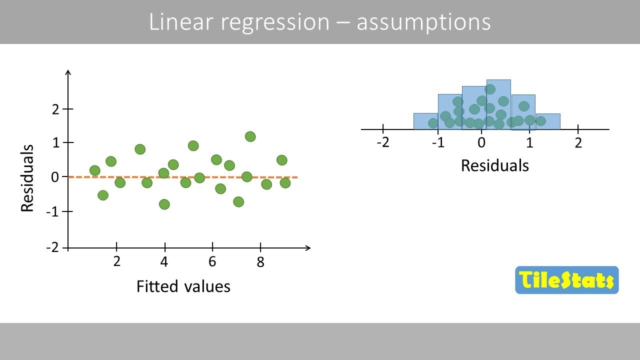
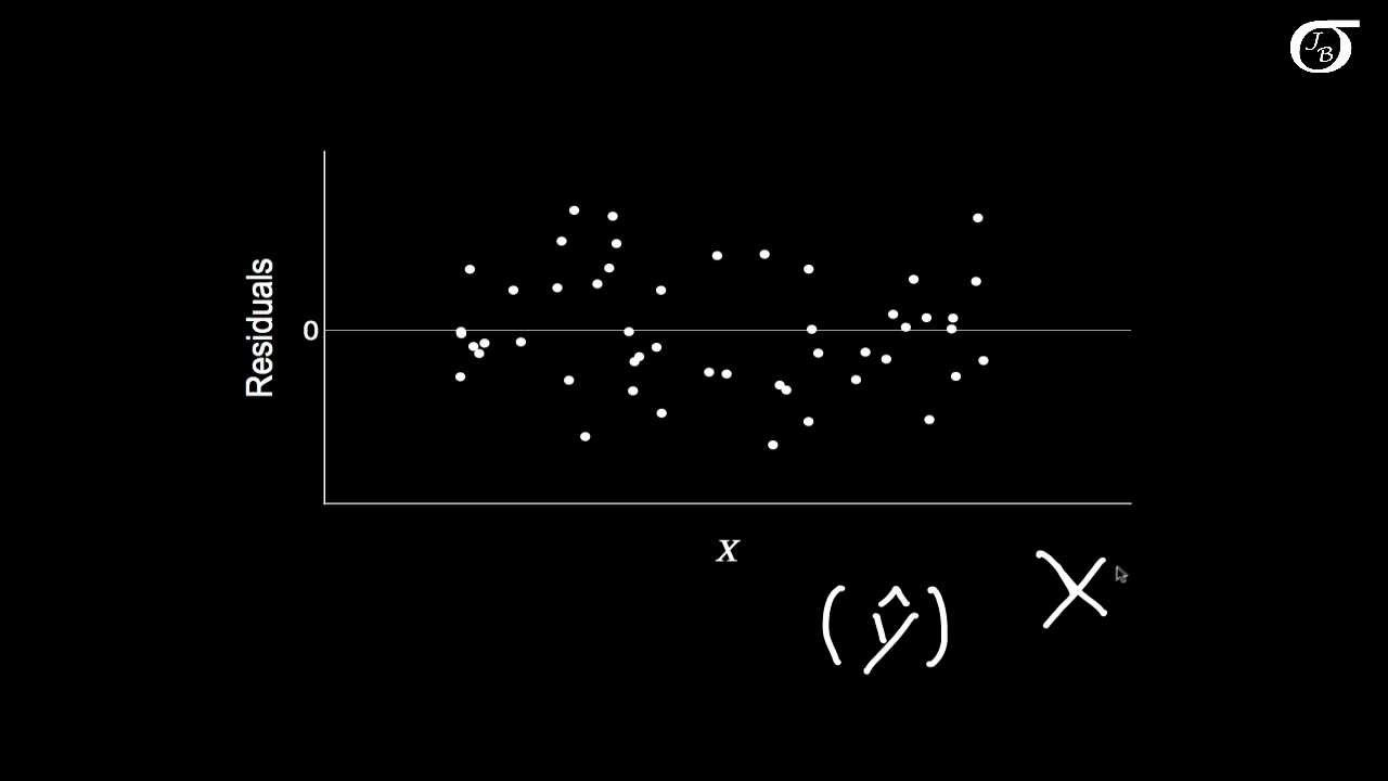
- 📋 Four key assumptions of Linear Regression are discussed: independence of Y values, linearity, homoscedasticity, and normal distribution of errors.
- 📊 R's built-in regression diagnostic plots help check these assumptions, with the first plot being the Residual plot.
- 📈 The QQ plot (Quantile-Quantile plot) checks if residuals are normally distributed, with points expected to fall on a diagonal line.
- 🛠️ The 'mfrow' command is used to display all four diagnostic plots on one screen for easier comparison.
- 🔬 Non-constant variance is indicated by a megaphone shape in the residual plot, suggesting increasing variance with larger predicted values.
- 🌐 Non-linearity in the relationship between variables is evident from a curved pattern in the residual plot and other diagnostic plots.
- 🔑 The importance of diagnostic plots is highlighted for checking assumptions in multiple linear regression models where scatterplots are not feasible.
Q & A
What is the main purpose of the video?
-The main purpose of the video is to introduce how to check the validity of the assumptions made when fitting a Linear Regression Model.
Why is it important to check the assumptions of a Linear Regression Model?
-It is important to check the assumptions because while the assumptions are never perfectly met, we need to ensure they are reasonable enough to work with, which helps in validating the model's reliability and accuracy.
What data set is used in the video to demonstrate the process?
-The LungCapacity data set is used in the video to demonstrate how to check the assumptions of a Linear Regression Model.
What is the dependent variable in the model discussed in the video?
-Lung Capacity is the dependent variable, also known as the outcome variable, in the model discussed in the video.
How is a Linear Regression Model typically fitted in R?
-A Linear Regression Model is typically fitted in R using the 'lm' command, which allows you to specify the dependent and independent variables.
What does the 'summary' command in R provide after fitting a model?
-The 'summary' command in R provides estimates of the model's slope and intercept, along with other summaries that help in understanding the model's performance.
What is the meaning of Y hat (Y^) in the context of the video?
-In the context of the video, Y hat (Y^) represents the predicted or fitted Y value, which is the mean of Y given X.
What are residuals in the context of a Linear Regression Model?
-Residuals are the differences between the observed Y values and the predicted or fitted Y values, and they are labeled with an 'e' in the video.
Why are residuals important in checking model assumptions?
-Residuals are important because they provide insights into the model's fit and help in checking the assumptions such as linearity, homoscedasticity, and normality of the error terms.
What is the purpose of the built-in regression diagnostic plots in R?
-The built-in regression diagnostic plots in R are used to visually assess the validity of the assumptions made when fitting a linear regression model, such as checking for linearity, homoscedasticity, and normality of residuals.
What does a 'megaphone shape' in a residual plot indicate?
-A 'megaphone shape' in a residual plot suggests that the variance is increasing, indicating a violation of the homoscedasticity assumption.
What does a curved pattern in the residual plot of a Linear Regression Model imply?
-A curved pattern in the residual plot implies a non-linear relationship between the variables, indicating a violation of the linearity assumption.
Why are diagnostic plots useful when dealing with multiple regression models?
-Diagnostic plots are useful in multiple regression models because they allow us to check the validity of the assumptions when we have too many variables to visualize the relationship between them, unlike in simple linear regression.
What is the significance of the QQ plot in regression diagnostics?
-The QQ plot, or quantile-quantile plot, is significant as it helps in assessing the normality of the residuals. If the residuals are normally distributed, the points in the QQ plot should fall roughly on a diagonal line.
Outlines
📊 Introduction to Linear Regression Assumptions
In this segment, Mike Marin introduces the importance of validating assumptions made during the fitting of a Linear Regression Model. He explains that while these assumptions are never perfectly met, it is essential to ensure they are reasonable enough to work with. The video uses the LungCapacity dataset to demonstrate the process of checking these assumptions. The focus is on the relationship between Age and Lung Capacity, with Lung Capacity as the dependent variable. A Scatterplot is used to visualize this relationship, and a Linear Regression Model is fitted using the 'lm' command in R. The summary of the model is then examined to understand the slope, intercept, and other statistical summaries. The concept of residuals and their standard deviation, known as the Residual Standard Error, is introduced as a tool for checking model assumptions.
🔍 Analyzing Model Residuals for Assumption Validation
This paragraph delves into the examination of model residuals to validate the assumptions of a Linear Regression Model. The assumptions discussed include independence of Y values, linearity, homoscedasticity, and normal distribution of errors. The video demonstrates how to use R's built-in regression diagnostic plots to check these assumptions. Four diagnostic plots are mentioned, which include the Residual plot, QQ plot, and two additional plots that help identify non-linearity and non-constant variance. The 'mfrow' command is introduced to display all four plots simultaneously. The video also addresses the importance of these diagnostic plots, especially in multiple linear regression where visualizing relationships between variables is not possible due to the high dimensionality.
📉 Detecting Non-constant Variance and Non-linearity
In this part of the video, Mike Marin discusses how to identify non-constant variance and non-linearity in a dataset. He presents an example dataset with increasing variance and fits a regression model called model2. The diagnostic plots for this model reveal a megaphone shape in the residual plot, indicating increasing variance with larger predicted values. The linearity assumption is confirmed to be met as the red line in the plot remains flat. The QQ plot shows normal distribution of residuals. Another dataset with a non-linear relationship is then introduced, and a linear model, model3, is fitted to it. The diagnostic plots for this model show a curved pattern in the residual plot, indicating non-linearity. The QQ plot confirms the normal distribution of residuals, but the non-linearity is evident in the other diagnostic plots. The video concludes by emphasizing the utility of diagnostic plots in checking model assumptions, especially in complex models with multiple variables.
Mindmap
Keywords
💡Linear Regression Model
💡Assumptions
💡Lung Capacity Data
💡Scatterplot
💡lm Command
💡Summary
💡Residuals
💡Residual Standard Error
💡Regression Diagnostic Plots
💡Homoscedasticity
💡Normal Distribution
💡mfrow Command
💡Non-linear Relationship
💡Multiple Linear Regression
Highlights
Introduction to checking the validity of assumptions in a Linear Regression Model.
Importing and attaching the LungCapacity dataset for analysis.
Explaining the relationship between Age and Lung Capacity as the dependent variable.
Using the 'plot' command to create a Scatterplot of Age vs Lung Capacity.
Fitting a Linear Regression Model with the 'lm' command and storing it as MOD.
Using 'summary' to get model estimates for Slope and Intercept.
Adding a regression line to the plot with the 'abline' command.
Defining Y hat as the predicted or fitted Y value and its formula.
Describing residuals as the difference between observed and predicted Y values.
The importance of the Residual Standard Error in understanding error size.
Assumptions of independence, linearity, homoscedasticity, and normal distribution of errors.
Using R's built-in regression diagnostic plots for assumption checking.
Interpreting the Residual plot for linearity and constant variation.
Understanding the QQ plot for normal distribution of residuals.
Using 'mfrow' to display all four diagnostic plots on one screen.
Identifying non-constant variance in a residual plot with a megaphone shape.
Demonstrating non-linearity in a scatterplot and its effect on diagnostic plots.
The utility of diagnostic plots in multiple linear regression with many variables.
Preview of the next video discussing further examination of model fit.
Transcripts
Browse More Related Video
Multiple Linear Regression in R | R Tutorial 5.3 | MarinStatsLectures
Assumptions in Linear Regression - explained | residual analysis

Regression diagnostics and analysis workflow

Simple Linear Regression in R | R Tutorial 5.1 | MarinStatsLectures

10.2.6 Regression - Residual Plots and Their Interpretation
Simple Linear Regression: Checking Assumptions with Residual Plots
5.0 / 5 (0 votes)
Thanks for rating: