Simple Linear Regression: Checking Assumptions with Residual Plots
TLDRThis script delves into the importance of validating assumptions in simple linear regression through residual plots. It explains that errors (epsilon) are expected to be normally distributed, homoscedastic, and independent. The script emphasizes checking these assumptions by observing the behavior of observed residuals, which should scatter randomly around the mean if the model's assumptions hold true. Various scenarios are discussed, including constant variance violation and systematic curvature in residuals, indicating model issues. The script also touches on potential solutions like weighted regression or model transformations. Real-world datasets are used to illustrate how residual plots can guide model refinement.
Takeaways
- 📊 In simple linear regression, the relationship between Y and X is assumed to be linear, with epsilon representing the random error component.
- 🧐 The error terms (epsilon) are assumed to be normally distributed, homoscedastic (equal variance), and independent.
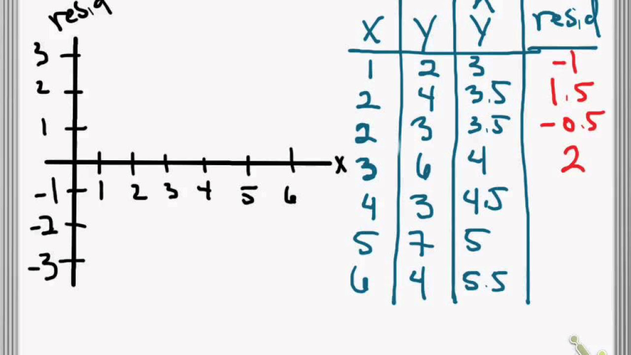
- 🔍 To validate these assumptions, one should investigate the behavior of the observed residuals (e_i), which is the difference between the actual and predicted Y values.
- 📈 When plotting residuals, they should be plotted against X or the predicted values (Y-hat), but not against the observed Y values to avoid misleading analysis.
- 🎯 In a valid linear regression model, the observed residuals should be approximately normally distributed and exhibit constant variance across different X values.
- 🚫 A residual plot should not show any systematic patterns, such as curvature or changes in variability, which could indicate issues with the model's assumptions.
- 🔢 The sum of residuals in a simple linear regression model is always zero, with a mean of zero, providing a quick visual check for the model's assumptions.
- ⚠️ If the residual plot shows increasing variance with X (heteroscedasticity), it violates the constant variance assumption and may require weighted regression or other adjustments.
- 📉 Systematic curvature in the residual plot suggests that the assumed linear relationship between Y and X may not be appropriate, and the model may need to be revised.
- 🕒 For time-series data, plotting residuals against time order can reveal issues not captured in the model, such as time-dependent effects that need to be addressed.
Q & A
What is the purpose of checking model assumptions with residual plots in simple linear regression?
-The purpose of checking model assumptions with residual plots in simple linear regression is to validate whether the assumptions about the random error term, such as normal distribution, homoscedasticity, and independence, hold true for the observed residuals. This helps in determining the validity of the model and the reliability of the statistical inferences made from it.
What does epsilon represent in the context of simple linear regression?
-In the context of simple linear regression, epsilon represents the random error component. It accounts for the variability in the dependent variable (Y) and is the difference between the actual observed value of Y and the predicted value from the regression line.
What are the key assumptions made about the error term in simple linear regression?
-The key assumptions made about the error term in simple linear regression are that the errors are normally distributed, homoscedastic (having equal variance for all values of X), and independent of each other.
How does the behavior of observed residuals indicate if the model assumptions are true?
-If the model assumptions are true, the observed residuals should be approximately normally distributed, have constant variance across different values of X, and show no systematic pattern. A random scattering of points around the horizontal axis indicates that the assumptions are likely valid.
Why is it important to plot residuals against X or predicted values (Y-hat) instead of observed values of Y?
-Plotting residuals against observed values of Y would be misleading because the residuals are calculated as the difference between the observed Y values and the predicted Y values. This would result in a perfect negative correlation and does not provide useful information about the model's performance.
What does it mean when the residuals sum to zero in a simple linear regression?
-In a simple linear regression, the residuals sum to zero because the model is designed to minimize the sum of squared residuals. This property provides a check on the model fit and is expected in a well-fitted linear regression.
What is the significance of systematic curvature observed in a residual plot?
-Systematic curvature in a residual plot indicates that the assumed linear relationship between the dependent and independent variables may not be appropriate. This could suggest the need for a more complex model, such as one with a polynomial term or a transformation of the variables.
What is weighted regression, and how does it address the issue of increasing variance with X?
-Weighted regression is a modification of the standard linear regression model where the observations are given different weights to account for the heteroscedasticity (unequal variance). By assigning weights that are inversely proportional to the variance, it can help to stabilize the variance across different values of X and improve the model fit.
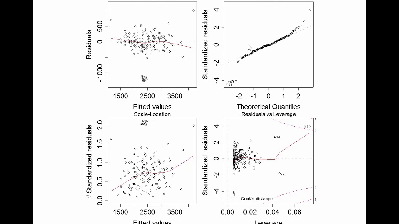
What does a normal quantile-quantile (Q-Q) plot indicate about the distribution of residuals?
-A normal Q-Q plot is used to assess the normality of the residuals. If the residuals are approximately normally distributed, the points on the Q-Q plot will form a straight line. Deviations from this line indicate that the residuals may not follow a normal distribution.
How can a residual plot against time order reveal issues with the model?
-A residual plot against time order can reveal patterns or trends in the residuals that were not accounted for in the model. If the residuals alternate between small and large values in a systematic way over time, it suggests that there may be a time-related effect or a serial correlation that has not been properly included in the model.
What actions can be taken if a residual plot indicates problems with the assumed model?
-If a residual plot indicates problems with the assumed model, one can consider transformations of the variables, adding polynomial terms, or using different types of regression models (e.g., weighted regression, non-linear models) to address the issues. Further investigation into the data and the relationships between variables may also be necessary to improve the model fit.
Outlines
📊 Investigating Model Assumptions with Residual Plots in Simple Linear Regression
This paragraph discusses the process of checking the assumptions of a simple linear regression model using residual plots. It explains that the model assumes a linear relationship between the dependent variable (Y) and the independent variable (X), with epsilon representing the random error term. The assumptions include normal distribution, homoscedasticity, and independence of error terms. The paragraph emphasizes the importance of investigating these assumptions, as they are crucial for statistical inference. It describes how observed residuals should behave if the model's assumptions hold true, and provides an example of plotting residuals against X or predicted values (Y-hat), but not against observed Y values, to avoid misleading results. The paragraph also highlights that in simple linear regression, residuals sum to zero and should display a random scattering of points without any indication of model assumption violations. It concludes by presenting different types of residual plots, each with varying levels of adherence to the model's assumptions, and suggests potential remedies for certain violations, such as weighted regression or using different models.
🧠 Activation Levels and Empathic Concern: A Residual Plot Analysis
This paragraph presents an analysis of activation levels in pain centers of the brain versus scores on the empathic concern scale for 16 women, using a residual plot. The least squares regression line is plotted, and the residual plot is examined for any signs of model assumption violations. The analysis finds no obvious problems, as there is no systematic curvature, and no major outliers are observed. It notes a potential minor variance in the residuals' distribution but does not consider it a significant issue. The paragraph then introduces a normal quantile quantile plot to further assess the normality of the residuals, concluding that they are approximately normally distributed. The residual plot and the quantile plot together indicate that the model's assumptions are reasonable, allowing for the application of statistical inference techniques.
Mindmap
Keywords
💡Simple Linear Regression
💡Residual Plots
💡Error Terms
💡Normal Distribution
💡Homoscedasticity
💡Independence
💡Variance
💡Curvature
💡Outliers
💡Weighted Regression
💡Time Order
Highlights
Investigating the assumptions of a simple linear regression model through residual plots.
The error term (epsilon) in the model is assumed to be normally distributed and homoscedastic, indicating equal variance and independence.
Observed residuals should behave similarly to the assumed error term if the model's assumptions are true.
Residuals should be approximately normally distributed with constant variance across different X values.
Plotting residuals against X or predicted values (Y-hat) is recommended over plotting against observed Y values to avoid misleading results.
In simple linear regression, residuals always sum to zero, providing a mean of zero.
A random scattering of residuals points indicates that the model's assumptions may be valid.
Systematic curvature or increasing variance in residuals with X indicates a violation of the model's assumptions.
Weighted regression can be used to address situations where variance increases with the mean.
Systematic curvature in residuals suggests that the assumed linear relationship may not be reasonable.
Recording observations in time order and plotting residuals against time can reveal unaccounted time effects.
Activation level in the pain centres of the brain versus empathic concern scale for women showed no obvious problems in the residual plot.
Jansko hardness versus density for Australian trees dataset showed potential issues with the assumed model, indicated by systematic curvature in the residual plot.
Improving the model may involve adding a X^2 term or transforming variables to achieve a straight-line relationship.
Normal quantile quantile plot can confirm if residuals are approximately normally distributed.
Transcripts
Browse More Related Video

10.2.6 Regression - Residual Plots and Their Interpretation

Residual plots | Exploring bivariate numerical data | AP Statistics | Khan Academy
Checking assumptions of the linear model

Checking Linear Regression Assumptions in R | R Tutorial 5.2 | MarinStatsLectures
Residuals and Residual Plots

How to Calculate the Residual
5.0 / 5 (0 votes)
Thanks for rating: