5.7 Numerical Integration (Quadrature)
TLDRThis video script delves into numerical integration, also known as quadrature, offering an applied mathematics perspective. It introduces three primary integration rules: the trapezoid rule, Simpson's rule, and Gaussian quadrature. The presenter explains these methods, emphasizing their ease of implementation and computational efficiency. The script also discusses error analysis in numerical integration, illustrating how the error decreases with an increase in integration points and comparing the performance of the different rules. The goal is to empower viewers to numerically integrate most functions and understand the abstract concept of integration.
Takeaways
- 📚 The lecture introduces numerical integration, emphasizing its practical applications in applied mathematics and its difference from analytical integration.
- 🔍 The concept of numerical integration is likened to a 'numerical recipe' that empowers students to integrate most functions numerically after mastering the material.
- 📈 The lecture explains the term 'quadrature', relating it to the historical method of counting boxes under a curve to approximate integrals.
- 📉 The Riemann definition of an integral is highlighted as the foundation for numerical integration algorithms, which essentially involve summing areas of infinitesimally small boxes.
- 📝 The importance of weights in numerical integration is discussed, with different methods for determining these weights to be introduced.
- 📋 Three main rules for numerical integration are presented: the trapezoid rule, Simpson's rule, and Gaussian quadrature, with the Monte Carlo method mentioned for multi-dimensional integrals.
- 📏 The trapezoid rule is detailed as the simplest method, approximating the integrand with straight lines and calculating areas of trapezoids.
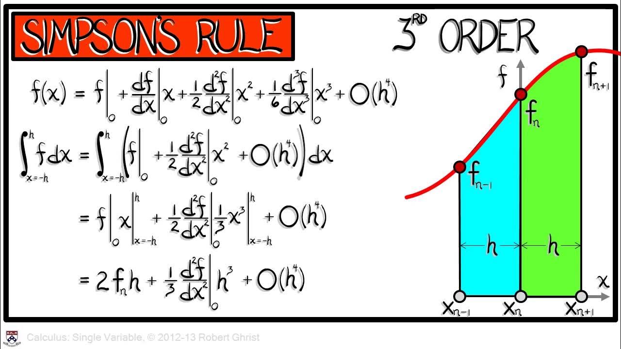
- 📐 Simpson's rule is introduced as a more accurate method using parabolic approximations over two intervals, requiring an odd number of points for integration.
- 🌟 Gaussian quadrature is highlighted as the 'golden rule', offering high accuracy by fitting a polynomial of degree 2n-1 using n evaluation points, typically chosen at the zeros of the Legendre polynomials.
- 📊 The lecture discusses the empirical analysis of integration errors, emphasizing the importance of understanding and balancing algorithmic error and round-off error in numerical computations.
- 📈 A practical approach to finding the optimal number of integration points is suggested, which involves balancing the approximation error with the round-off error to achieve the best precision.
Q & A
What is numerical integration and how does it differ from analytical integration?
-Numerical integration is a method used to calculate the integral of a function numerically, often using algorithms like the trapezoid rule or Simpson's rule. It differs from analytical integration, which involves finding an exact expression for the integral using calculus. Numerical integration is often easier to perform on a computer and is used when an analytical solution is difficult to obtain or does not exist.
What is the quadrature in the context of numerical integration?
-Quadrature refers to the process of numerical integration. The term originates from the Latin word for 'fourth power' and is historically related to the use of counting squares (or boxes) under a curve to approximate the area, which represents the integral of the function.
What is the Riemann definition of an integral and how is it used in numerical integration?
-The Riemann definition of an integral states that the definite integral from a to b of a function is the limit of the sum of the product of the function values at n points within the interval and the width of the box (h) as n approaches infinity and h approaches zero. In numerical integration, this definition is used as the basis for algorithms, but instead of taking the limit, finite values of n and h are used to approximate the integral.
How does the trapezoid rule approximate the integral of a function?
-The trapezoid rule approximates the integral by dividing the area under the curve into trapezoidal shapes. It calculates the area of each trapezoid by taking the average of the function values at the endpoints of each interval and multiplying by the interval width (h), then summing these areas to estimate the integral.
What is Simpson's rule and how does it differ from the trapezoid rule?
-Simpson's rule is another method for numerical integration that approximates the integral by fitting parabolas between intervals of the function instead of straight lines as in the trapezoid rule. It is generally more accurate than the trapezoid rule but requires an even number of intervals and involves more complex calculations for the weights applied to each function evaluation.
What is the significance of Gaussian quadrature and how does it work?
-Gaussian quadrature is a highly accurate numerical integration method that is often used by scientists and engineers. It involves choosing specific points (usually the zeros of orthogonal polynomials) and corresponding weights to evaluate the function, which allows for exact integration of polynomials up to a certain degree and provides excellent approximation for other functions.
Why is it important to understand the errors in numerical integration?
-Understanding errors in numerical integration is crucial because it helps determine the accuracy and reliability of the results. Errors can arise from approximation (how well the method fits the function) and round-off (due to the finite precision of computer calculations). Knowing the error behavior helps in choosing the optimal number of points for a given level of accuracy.
How can one determine the optimal number of points for a numerical integration method?
-The optimal number of points can be determined experimentally by comparing the approximation error (which decreases with more points) and the round-off error (which increases with more points due to accumulation). The best number of points is typically where these two types of errors balance each other out, providing the most accurate result.
What is the relationship between the number of points used in an integration method and the error of the method?
-The error of an integration method typically decreases as the number of points increases. For the trapezoid rule, the error decreases with the square of the number of points (1/n^2), while for Simpson's rule, it decreases even faster (1/n^4). Gaussian quadrature has an even faster falloff rate, making it highly accurate.
What challenges might one encounter when trying to integrate functions that give results close to zero?
-When integrating functions that result in values close to zero, numerical methods can struggle due to the difficulty of accurately calculating small numbers. This can lead to large relative errors, as dividing by a small number (or zero) can result in very large error values. Additionally, round-off errors can become more significant in these cases.
Outlines
📚 Introduction to Numerical Integration
The speaker introduces the topic of numerical integration, emphasizing its practical applications in applied mathematics. They highlight the difference between numerical and analytical integration, noting that the former is more straightforward. The lecture aims to empower students to integrate a wide variety of functions numerically and to deepen their understanding of the concept of integration. The speaker also introduces the term 'quadrature', relating it to the historical method of counting squares under a curve to approximate an integral's value.
📐 The Basics of Numerical Integration Techniques
This paragraph delves into the specifics of numerical integration methods, starting with the simple act of 'counting boxes' to approximate integrals. It explains the importance of accurately treating the top of these boxes to improve integration rules. The speaker references the Riemann definition of an integral, which is the foundation for numerical integration algorithms. They describe how these algorithms work by summing the product of function values at certain points and weights, which are typically fractions of the box height.
📉 Exploring the Trapezoid Rule for Numerical Integration
The speaker presents the trapezoid rule, a numerical integration method that approximates the function with straight lines. They discuss how to calculate the area under a trapezoid by averaging the heights at the ends and multiplying by the width. The paragraph explains the process of summing these areas for multiple trapezoids to approximate the integral over an interval, emphasizing the simplicity and uniform step size of this method.
📈 Simpson's Rule and Parabolic Approximations
Simpson's rule is introduced as an improvement over the trapezoid rule, using parabolic fits instead of straight lines. The speaker explains the requirement for an even number of intervals and an odd number of points for this method. They detail the process of fitting parabolas to the function across two intervals and calculating the area under each parabola, then summing these areas with specific weights to approximate the integral.
🌟 Gaussian Quadrature: The Advanced Integration Technique
Gaussian quadrature is introduced as an advanced and highly effective integration rule. The speaker explains that it involves fitting a high-degree polynomial to the function using the points and weights determined by Gauss. These points are the zeros of the Legendre polynomials, and the weights are related to the derivative of the Legendre polynomial at these zeros. The method is praised for its accuracy and is commonly used by working scientists.
📊 Analyzing Errors in Numerical Integration
The speaker discusses the concept of integration errors, defining relative error and its significance in computational science. They explain how to analyze errors by taking the logarithm of the error to determine the number of significant figures. The paragraph includes a discussion of approximation error and round-off error, showing how these errors can be visualized and analyzed using a log-log plot. The speaker emphasizes the importance of understanding when to stop increasing the number of integration points to balance between computational efficiency and accuracy.
🔍 Optimal Number of Points for Integration
This paragraph focuses on determining the optimal number of points for numerical integration, balancing between the decreasing algorithmic error and the increasing round-off error. The speaker provides a method to set the two types of errors equal to each other and solve for the best value of n, the number of points. They illustrate this with examples from the trapezoid and Simpson rules, showing how the Simpson rule achieves higher precision with fewer points due to less opportunity for round-off error to accumulate.
🧪 Empirical Error Analysis in the Lab
The speaker encourages students to conduct their empirical error analysis using the integration rules learned, such as the trapezoid, Simpson, and Gaussian quadrature. They suggest integrating functions like e^(-x) and x^2 * e^(-x) from 0 to 1 to understand the error behavior. The paragraph guides students to plot the error against the number of points on a log-log scale, deduce the slope, and compare it with theoretical predictions. The speaker also challenges students to try more complex cases, like integrating a sine wave or a function with a rapidly oscillating component.
🚀 Conclusion and Final Challenges
In conclusion, the speaker highlights the importance of practical application of numerical integration techniques and the challenges associated with integrating functions that result in zero or near-zero values. They caution about the difficulty of accurately calculating such integrals and the limitations of even the most powerful computers. The speaker ends with an invitation for students to explore these challenges further, encouraging them to enjoy the process of computation and numerical integration.
Mindmap
Keywords
💡Numerical Integration
💡Applied Mathematics
💡Quadrature
💡Riemann Sum
💡Trapezoid Rule
💡Simpson's Rule
💡Gaussian Quadrature
💡Monte Carlo Method
💡Error Analysis
💡Significant Figures
Highlights
Introduction to numerical integration as a powerful tool in applied mathematics, distinct from analytical integration.
Numerical integration likened to a 'numerical recipe' that simplifies the process of integration.
Emphasis on the practicality of numerical integration for solving a wide range of problems.
Explanation of 'quadrature' as an old English term related to numerical integration through counting boxes under a curve.
The Riemann definition of an integral as the foundation for numerical integration algorithms.
Discussion on the importance of the choice of weights in numerical integration methods.
Introduction of the trapezoid rule as the simplest numerical integration method using straight lines.
Simpson's rule explained as a more accurate method using parabolic approximations.
Gaussian quadrature presented as the 'golden rule' for its high accuracy in integration.
The significance of Gaussian quadrature in fitting high-degree polynomials for better integration results.
Error analysis in numerical integration, including the impact of round-off errors.
The relationship between the number of integration points and the accuracy of the result.
Practical advice on choosing the optimal number of points for numerical integration.
The importance of understanding the limitations of numerical integration methods.
Hands-on application of numerical integration rules in a lab setting for empirical error analysis.
Challenges of integrating functions that yield zero or near-zero results due to computational inaccuracies.
Encouragement for students to explore and experiment with numerical integration methods.
Transcripts
Browse More Related Video

Numerical Integration - Trapezoidal Rule & Simpson's Rule

Numeric Integration with Python — Topic 89 of Machine Learning Foundations
Calculus Chapter 5 Lecture 49 Numerical Integration II

Numerical Integration With Trapezoidal and Simpson's Rule

Lec 25 | MIT 18.01 Single Variable Calculus, Fall 2007
Rules for Integration
5.0 / 5 (0 votes)
Thanks for rating: