Logistic Growth
TLDRIn this lesson, we explore logistic growth, a model that differs from exponential growth. Unlike exponential graphs, logistic graphs start like a rocket but form an S-curve, indicating a limit due to resource constraints. This limit, or horizontal asymptote, represents the maximum population. The inflection point, where concavity changes, occurs at half this limit. The lesson covers solving differential equations to find these points, graphing logistic curves, and analyzing the concavity and behavior of these curves under different initial conditions. Students will practice these concepts in the next session.
Takeaways
- 📈 The script introduces logistic growth as a model for population growth with limited resources, contrasting it with exponential growth.
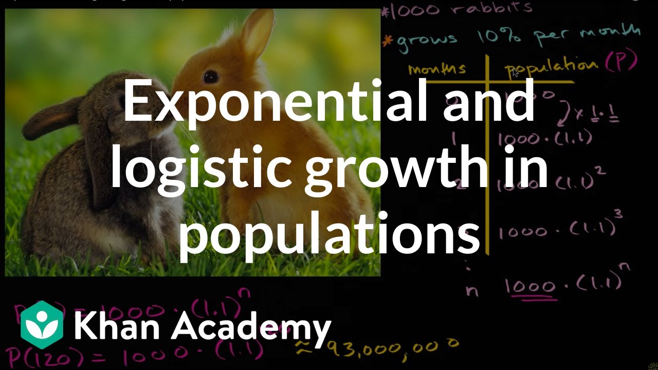
- 🚀 Exponential growth graphs typically pass through the point (0,1) and can increase rapidly, while logistic growth also starts rapidly but eventually levels off.
- 🔄 Logistic growth models change concavity and have an 'S' shaped curve, indicating a point of inflection where the growth rate changes.
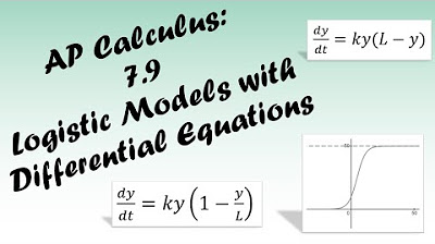
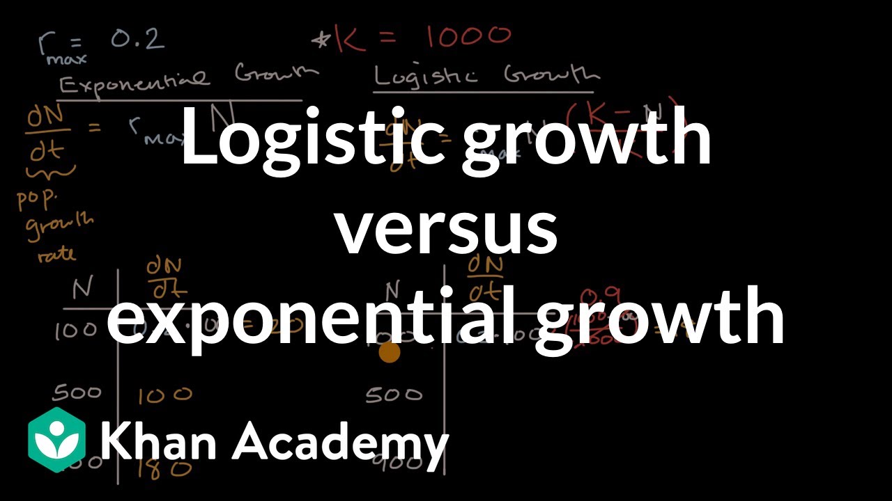
- 📚 The logistic growth differential equation is given by dp/dt = r * P * (1 - P/L), where r is the growth rate, P is the population, and L is the carrying capacity.
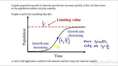
- 🔍 The carrying capacity (L) is the horizontal asymptote of the logistic growth curve, representing the maximum population size the environment can sustain.
- 📉 The point of inflection in a logistic growth curve occurs at P = L/2, which is halfway to the carrying capacity.
- 📌 The range of the solution curve for logistic growth is from the initial population size to the carrying capacity, but never reaching it.
- 📈 The population is increasing when P is between the initial population and the carrying capacity, as dp/dt is positive in this range.
- 📊 The concavity of the logistic growth curve changes at the inflection point; it is concave up below the midpoint and concave down above it.
- 🔢 The second derivative, d²P/dt², helps determine concavity, with positive values indicating concave up and negative values indicating concave down.
- 🐟 An example given in the script uses a differential equation dp/dt = 3P(1 - P/6000) to illustrate how to manipulate and analyze logistic growth models.
Q & A
What is logistic growth?
-Logistic growth is a model that describes population growth under limited resources. Unlike exponential growth, it increases rapidly at first but eventually slows down and reaches a plateau, known as the carrying capacity.
How does logistic growth differ from exponential growth?
-Exponential growth continues to increase without bound, often represented by a graph that goes through the point (0,1) and rapidly increases. Logistic growth, on the other hand, starts similarly but eventually levels off, reaching a maximum population size called the carrying capacity.
What is the carrying capacity in the context of logistic growth?
-The carrying capacity is the maximum population size that the environment can sustain indefinitely. In logistic growth, the population growth rate slows as the population approaches this limit.
What is the significance of the point of inflection in logistic growth?
-The point of inflection is where the graph of logistic growth changes concavity. It is significant because it indicates a shift in the rate of population growth, from accelerating to decelerating.
What is the formula for logistic growth?
-The logistic growth differential equation is given by \( \frac{dp}{dt} = r \cdot p \cdot (1 - \frac{p}{K}) \), where \( p \) is the population, \( K \) is the carrying capacity, and \( r \) is the intrinsic growth rate.
How do you determine the carrying capacity from the logistic growth equation?
-The carrying capacity \( K \) can be determined from the logistic growth equation by identifying the term that is subtracted from 1 in the equation. In the given example, \( K \) is 18,000.
What does the range of the solution curve represent in logistic growth?
-The range of the solution curve in logistic growth represents the possible values of the population, from the initial population to the carrying capacity.
How does the initial population size affect the logistic growth curve?
-The initial population size affects the starting point of the logistic growth curve but does not change the carrying capacity. If the initial population is higher, the curve will start higher and approach the carrying capacity from above.
What is the significance of the second derivative in determining concavity in logistic growth?
-The second derivative indicates whether the curve is concave up or concave down. If the second derivative is positive, the curve is concave up; if it is negative, the curve is concave down.
What happens when the population exceeds the carrying capacity in logistic growth?
-If the population exceeds the carrying capacity, the growth rate becomes negative, and the population decreases. The curve will be concave up in this scenario, indicating an increasing rate of decrease.
Outlines
📈 Introduction to Logistic Growth
The video script begins with an introduction to logistic growth, contrasting it with exponential growth. It explains that while exponential growth can be represented by a graph that shoots up from the origin, logistic growth starts similarly but then levels off, forming an 'S' curve. This is due to limited resources that affect population growth. The script introduces the logistic growth model equation, dp/dt = rP(1 - P/K), where r is the growth rate, P is the population, and K is the carrying capacity or limit. An example is given with a differential equation, and the process of factoring to simplify the equation is demonstrated. The script also discusses the range of the solution curve and how to determine when the population is increasing or decreasing by analyzing the first derivative, dp/dt.
🔍 Analyzing Concavity and Inflection Points
The second paragraph delves into the analysis of concavity and inflection points in logistic growth. It explains how to find the second derivative to determine concavity and locate the inflection point. The script uses the example from the previous paragraph to demonstrate how to calculate the second derivative and set it to zero to find the inflection point, which is at P = 9,000 in the given example. It then discusses how the sign of the second derivative changes at this point, indicating a switch from concave up to concave down. The script also explores the implications of different initial conditions on the shape of the logistic growth curve, such as starting with a population larger than the inflection point, which results in a curve that is always increasing and concave down.
📉 Impact of Overpopulation on Logistic Growth
The final paragraph of the script addresses the scenario of overpopulation in the context of logistic growth. It discusses what happens when the initial population exceeds the carrying capacity, leading to a decrease in the population towards the carrying capacity. The script explains that in this case, the first derivative becomes negative, indicating a decreasing population, while the second derivative is positive, indicating the curve is concave up. This results in a unique situation where the population is decreasing but the growth curve is concave up. The script concludes by summarizing the logistic growth model and its implications, and mentions that further practice will be done in the next session.
Mindmap
Keywords
💡Logistic Growth
💡Exponential Growth
💡Differential Equation
💡Carrying Capacity (L)
💡Point of Inflection
💡Concavity
💡Second Derivative
💡Horizontal Asymptote
💡Initial Conditions
💡Inflection Point
Highlights
Logistic growth is a model different from exponential growth, characterized by an S-curve and a change in concavity.
Exponential growth graphs usually pass through the point (0,1) and can increase or decrease rapidly.
A logistic graph starts with rapid growth like exponential but eventually levels off, forming an S-curve.
The logistic model is used to represent population growth with limited resources.
The limit of the logistic growth model is represented by a horizontal asymptote.
The point of inflection in a logistic graph occurs at half the limit of the population size.
The differential equation for logistic growth is given by dp/dt = r * P * (1 - P/L), where r is the growth rate, P is the population, and L is the limit.
The example provided demonstrates converting a logistic differential equation into the standard form by factoring.
The limit of the logistic growth model can be determined by setting the derivative equal to zero and solving for P.
The range of the solution curve for logistic growth is from the initial population to the limit, but never reaching the limit.
The solution curve for logistic growth is increasing when the population is between the initial value and half the limit.
The inflection point of the logistic curve is found by taking the second derivative and setting it to zero.
The concavity of the logistic curve changes at the inflection point, indicating a switch from concave up to concave down.
Graphing the logistic curve involves starting at the initial population, increasing until the inflection point, then leveling off towards the limit.
Changing initial conditions of the logistic model affects the starting point but not the limit or the overall shape of the curve.
If the initial population exceeds the inflection point, the logistic curve will always be increasing and concave down until it approaches the limit.
An excessive initial population results in a decreasing population towards the limit, starting concave up but eventually concave down.
Transcripts
Browse More Related Video
5.0 / 5 (0 votes)
Thanks for rating: