Logistic Growth Function and Differential Equations
TLDRThe video script delves into the concept of logistic equations, contrasting them with exponential growth. It explains that while exponential growth is limitless, logistic growth is capped by the carrying capacity, a concept exemplified by the population dynamics of a species on an island with limited resources. The script outlines the differential equations for both growth models and guides viewers through deriving the general logistic equation from the logistic differential equation using integration techniques and partial fraction decomposition. The logistic equation is then applied to a hypothetical scenario involving the population growth of dogs on an island, illustrating how to calculate the population at different times, estimate the year when the population reaches a certain threshold, and determine the annual birth rate. The video concludes with alternative methods for estimating population growth rates, emphasizing the average rate of change as a practical approximation for the instantaneous rate of change at a specific time point.
Takeaways
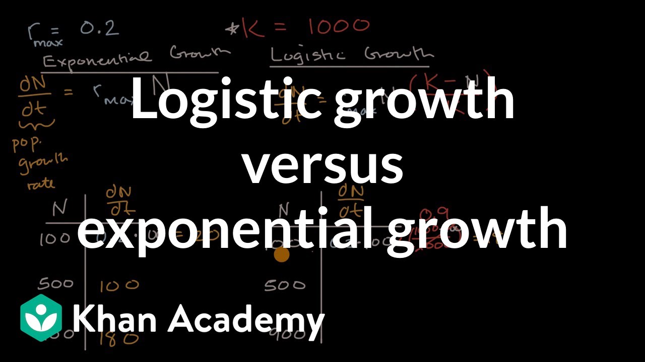
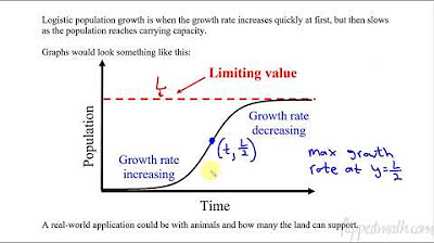
- 📈 The difference between exponential and logistic growth is that exponential growth is unlimited and increases at an increasing rate, while logistic growth is limited and reaches a maximum carrying capacity.
- 🧮 The differential equation for exponential growth is dy/dt = ky, whereas for logistic growth it is dy/dt = ky(1 - y/l), where l is the carrying capacity.
- 📌 In logistic growth, as the population size (y) approaches zero, the growth rate (dy/dt) approaches that of exponential growth, since y/l approaches zero.
- 🔁 When the population size (y) is close to the carrying capacity (l), the growth rate (dy/dt) approaches zero, indicating that the population growth levels off.
- 🌱 The general solution for an exponential growth curve is y = ce^(kt), and for a logistic curve, it is y = l/(1 + b*e^(-kt)), where b is a constant.
- ✅ To derive the logistic equation from the differential equation, integrate both sides after applying partial fraction decomposition and finding the antiderivatives.
- 🔍 The constants in the logistic equation can be determined by using known population values at specific times and solving the resulting system of equations.
- 📉 The logistic model is useful for describing population dynamics where resources are limited and the environment can only support a certain maximum population size.
- 🧮 To find the number of births per year, you can use the logistic differential equation and calculate the net growth by subtracting deaths from births.
- 📊 The average rate of change can approximate the instantaneous rate of change, especially when calculated over years close to the point of interest.
- ⏱️ The year when the population reaches a certain size can be found by solving for time (t) in the logistic growth equation when the population (p) is set to that size.
Q & A
What is the primary difference between exponential growth and logistic growth?
-Exponential growth increases at an increasing rate without limit, whereas logistic growth initially increases exponentially but then slows down, eventually reaching a maximum level known as the carrying capacity, beyond which the growth stops.
What is the carrying capacity (l) in the context of logistic growth?
-The carrying capacity (l) is the maximum population size that an environment can sustain indefinitely, representing the upper limit of growth in a logistic model.
What is the differential equation for exponential growth?
-The differential equation for exponential growth is given by dy/dt = k*y, where y is the population size, t is time, and k is the growth rate constant.
How does the logistic growth differential equation differ from that of exponential growth?
-The logistic growth differential equation is dy/dt = k*y * (1 - y/l), which includes an additional term (1 - y/l) that accounts for the carrying capacity limit, unlike the exponential growth equation.
What happens to the rate of population increase (dy/dt) as the population size (y) approaches the carrying capacity (l) in a logistic growth model?
-As the population size (y) approaches the carrying capacity (l), the term (y/l) approaches 1, making (1 - y/l) approach 0, and thus dy/dt approaches 0. This means the rate of population increase becomes zero, and the population stops growing.
What is the general solution for the logistic growth model in terms of y?
-The general solution for the logistic growth model is y = l / (1 + b * e^(-kt)), where l is the carrying capacity, k is the growth rate constant, b is another constant, and t is time.
How can you derive the general logistic equation starting from the logistic differential equation?
-You can derive the general logistic equation by first multiplying both sides of the logistic differential equation by dt and then dividing by y(1 - y/l), followed by integrating both sides with respect to their respective variables, and finally solving for y.
In the context of the logistic growth model, what does the constant b represent?
-The constant b in the logistic growth model represents the initial growth rate adjustment factor. It is derived from the integration process and is used to ensure that the logistic equation passes through the initial conditions of the problem.
How many dogs were estimated to be on the island by 2020 using the logistic growth model?
-By 2020, the logistic growth model estimated there to be approximately 1094 dogs on the island.
What is the net growth rate of the dog population in 2016, according to the logistic model?
-The net growth rate of the dog population in 2016 was approximately 94 dogs per year, which accounts for both births and deaths resulting in a net increase in population.
How can you approximate the instantaneous rate of change of the population in 2016 using the average rate of change formula?
-You can approximate the instantaneous rate of change in 2016 by calculating the average rate of change between two years that are close to 2016, such as 2015 and 2017, and taking the average of the population changes during those years.
Outlines
📈 Introduction to Logistic vs. Exponential Growth
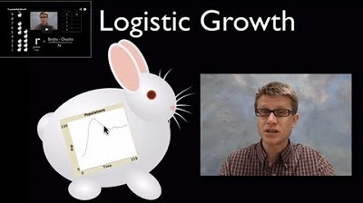
This paragraph introduces the topic of logistic equations and their general solution. It contrasts exponential growth, which increases without limit, with logistic growth, which starts to slow and eventually levels off, reaching a maximum called the carrying capacity. The logistic curve is particularly useful for modeling population growth, where resources are finite. The differential equations for both growth types are presented: exponential growth is represented by dy/dt = k*y, while logistic growth is given by dy/dt = k*y*(1 - y/l), where k is the growth rate and l is the carrying capacity.
🧮 Deriving the Logistic Growth Equation
The paragraph explains the process of deriving the logistic growth equation from its differential form. It begins by manipulating the logistic growth differential equation to separate variables and integrate. Using partial fraction decomposition, the equation is transformed into a form that allows for integration, leading to the general logistic equation y = l / (1 + b * e^(-kt)), where b is a constant to be determined. The process involves integrating both sides of the equation, applying properties of logarithms, and solving for the constants involved.
🔍 Partial Fraction Decomposition and Integration
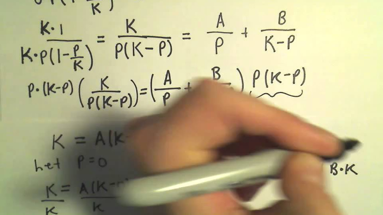
This section delves into the specifics of using partial fraction decomposition to simplify the logistic growth equation for integration. It demonstrates how to set up and solve for the constants a and b in the equation, leading to the discovery that both are equal to one. The paragraph concludes with the integrated form of the logistic equation, ready for further manipulation to find the general solution.
🧬 General Solution and Problem Application
The paragraph presents the general solution for the logistic equation and applies it to a problem involving dog population growth on an island. It outlines how to use the general logistic equation y = l / (1 + b * e^(-kt)) to create a specific equation for the dog population, denoted as p(t). Using given population data for the years 2005 and 2012, the constants b and k are solved for, allowing for the creation of a predictive model for the dog population at any given time t.
📚 Calculating Future Population and Growth Rate
This part of the script calculates the dog population on the island for the year 2020 and determines in what year the population will reach one thousand dogs. It involves plugging in values into the logistic growth equation and solving for time t when the population p(t) equals one thousand. The paragraph also explains how to calculate the number of dogs born per year in 2016 using the logistic differential equation.
📉 Estimating Annual Births and Deaths
The paragraph discusses how to estimate the number of dogs born and dying each year by analyzing the net growth of the population. It clarifies the difference between the number of dogs born and the net increase in population, which accounts for both births and deaths. The script provides a method to estimate the number of dogs dying in a year, given the birth rate and net growth.
📊 Approximating the Rate of Population Change
The final paragraph explores different methods to approximate the rate of population change. It demonstrates the use of the average rate of change formula to estimate the instantaneous rate of change at a specific year, using nearby years for a more accurate approximation. The script concludes with a summary of the various approaches to calculating and estimating population growth and change, reinforcing the concepts covered in the video.
Mindmap
Keywords
💡Logistic Equations
💡Exponential Growth
💡Logistic Growth
💡Carrying Capacity (L)
💡Differential Equation
💡General Solution
💡Partial Fraction Decomposition
💡Anti-Derivative
💡Natural Logarithm (ln)
💡Relative Growth Rate (k)
💡Net Growth
Highlights
The video focuses on logistic equations and their general solution derivation.
Differentiates between exponential growth and logistic growth, with exponential growth being unlimited and logistic growth having a carrying capacity.
Exponential growth is represented by the differential equation dy/dt = ky, while logistic growth is represented by dy/dt = ky(1 - y/l).
When y is small, the logistic curve behaves exponentially, but as y approaches the carrying capacity l, the growth rate decreases to zero.
The general solution for an exponential growth curve is y = ce^(kt), where c is a constant.
The general solution for a logistic growth curve is y = l / (1 + be^(-kt)), where l is the carrying capacity, k is the growth rate, and b is another constant.
Derivation of the logistic curve equation from the differential equation involves multiplying by dt, dividing by y(1 - y/l), and integrating both sides.
Partial fraction decomposition is used to help integrate the left side of the logistic differential equation.
The constants a and b in the partial fraction decomposition are both found to be equal to 1.
Integration of the logistic differential equation leads to the natural log property ln(a - ln(b)) = ln(a/b).
The general logistic equation is derived by separating variables and applying properties of exponents and natural logs.
An example problem is solved involving the logistic growth of a dog population on an island, with an initial population and a carrying capacity provided.
The values for b and k are solved using the initial and final population counts, allowing for the general logistic equation to be written for the dog population.
The population at a future time (2020) is calculated by substituting the known values into the logistic equation.
The year when the population reaches a specific target (1000 dogs) is found by solving the logistic equation for that population size.
The number of dogs born per year in 2016 is estimated using the logistic differential equation and the population size at that time.
The net growth of the population per year is explained to account for both births and deaths, providing a clearer picture of population dynamics.
An approximation method using the average rate of change over two years close to the year of interest is shown to estimate the instantaneous rate of population change.
The video concludes with a summary of the different methods used to calculate and approximate population growth rates in logistic models.
Transcripts
Browse More Related Video
5.0 / 5 (0 votes)
Thanks for rating:
