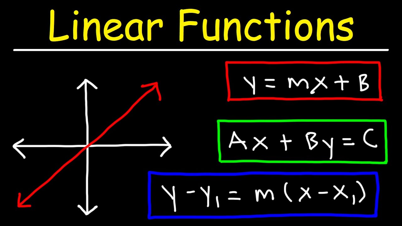
Ch. 2.5 Linear Functions and Models
TLDRThis video script covers chapter 2.5 on linear functions and models, focusing on solving word problems through linear equations. It explains the need for an initial value, slope, or two points to determine a line's equation. The script uses two examples: calculating the time until two people lose radio contact based on their walking speeds and directions, and predicting a town's population growth using historical data. It illustrates the process of formulating and solving linear equations to find answers to practical questions.
Takeaways
- 📚 The lesson is about linear functions and models, focusing on solving word problems related to linear equations.
- 🔍 To create a linear equation, one needs an initial value and a slope, a rate of change and a point, or two sets of input-output pairs.
- 📈 The concept of slope is crucial, representing a rate of change, which is the key to identifying linear relationships in word problems.
- 👥 The first example involves Rikako and Vitor walking in different directions, and the problem is about determining when they will be out of radio contact range.
- 📍 The problem-solving approach involves visualizing the scenario, identifying distances traveled by each person as functions of time, and setting up an equation based on the maximum allowable distance for radio contact.
- 🧩 The distance formula used in the example is the Pythagorean theorem, which is applied to find when the distance between Rikako and Vitor equals the radio range.
- 📊 The second example discusses the linear growth of a town's population, with data points from 2004 and 2009 to establish a trend.
- 📉 The population growth is modeled using a linear function derived from the given data points, allowing for predictions about future population sizes.
- 🔢 The slope of the population growth line is calculated by the change in population over the time span between the two data points.
- ⏱ The function is then used to predict the population in 2021 and to determine the year when the population will reach 15,000.
- 🔮 The method involves substituting the desired year into the function to find the corresponding population and solving the function for the year when the population target is met.
Q & A
What is the main topic of Chapter 2.5 in the video script?
-The main topic of Chapter 2.5 is linear functions and models, specifically focusing on solving word problems related to linear functions.
What prerequisite knowledge is assumed for understanding Chapter 2.5?
-The prerequisite knowledge assumed is from Chapter 1.10, where equations of lines and concepts such as slope and rate of change were discussed.
What are the three essential elements needed to create the equation of a line according to the script?
-The three essential elements needed are an initial value and a slope, a rate of change and a generic point (input-output pair), or two sets of inputs and outputs to find the rate of change.
How does the script define 'slope' in the context of linear functions?
-In the script, 'slope' is defined as a rate of change, which can be thought of as the amount of change per unit for a given input.
What is the first example problem discussed in the script?
-The first example problem involves Rikako and Vitor walking in different directions at different speeds and determining when they will lose radio contact based on the range of their two-way radio.
What is the mathematical formula used to calculate the distance between Rikako and Vitor in the first example?
-The formula used is the square root of the sum of the squares of their respective distances traveled, which is \( \sqrt{(4t)^2 + (3t)^2} \), where \( t \) is the time in hours.
What is the second example problem presented in the script?
-The second example problem is about predicting the population growth of a town based on its past population numbers in 2004 and 2009.
How is the linear model for the town's population growth derived in the script?
-The linear model is derived by using the two data points (2004 with a population of 6200 and 2009 with a population of 8100) to calculate the slope and then formulating the equation as \( 380t + 6200 \).
What is the predicted population of the town in 2021 according to the script?
-The predicted population in 2021 is 12,660, calculated by substituting \( t = 17 \) (years since 2004) into the derived linear model.
In what year will the town's population reach 15,000 according to the script?
-The town's population is predicted to reach 15,000 in the year 2027, which is approximately 23 years after 2004.
Outlines
📚 Introduction to Linear Functions and Word Problems
This section of the video introduces Chapter 2.5, which focuses on linear functions and models. The instructor emphasizes that this will be a brief segment, primarily addressing word problems related to linear functions. The foundation for understanding these problems was laid in Chapter 1.10, where the equations of lines were discussed. The key to solving these problems is identifying the necessary components to create a linear equation: an initial value and a slope, or a rate of change and a generic point, or two sets of input-output pairs to determine the rate of change. The first example involves Rikaku and Vitor walking in different directions with given speeds and a two-way radio with a limited range, aiming to determine when they will lose contact. The instructor illustrates the problem with a visual representation and uses the Pythagorean theorem to solve for the time when they will be out of range.
📈 Modeling Population Growth with Linear Functions
The second paragraph delves into a real-world application of linear functions by examining the linear growth of a town's population over time. The data provided includes the population in 2004 and 2009, from which the instructor calculates the constant growth rate. By considering the years since 2004 as a variable 't', a linear model is formulated to represent the population growth. The model is then used to predict the population for the year 2021 and to determine the year when the population will reach 15,000. The instructor demonstrates the process of solving for 't' in both scenarios, resulting in predictions for the future population and the specific year when the town's population will hit the 15,000 milestone.
Mindmap
Keywords
💡Linear Functions
💡Models
💡Word Problems
💡Equations of Lines
💡Initial Value
💡Slope
💡Rate of Change
💡Input and Output
💡Generic Point
💡Distance
💡Population Growth
Highlights
Introduction to Chapter 2.5 on linear functions and models.
Explanation that this section focuses on solving word problems related to linear functions.
Brief overview of prerequisite knowledge from Chapter 1.10 on equations of lines.
Description of the three essential elements needed to create a linear function: initial value, slope, or rate of change.
Emphasis on identifying the given information in word problems to determine the linear equation.
Illustration of the process to find the equation of a line using an example involving two people walking in different directions.
Use of a two-way radio example to explain how to determine when communication will be lost due to distance.
Introduction of the distance formula involving the square root of the sum of squared distances.
Solution to the problem of calculating the time when the two individuals will be out of radio contact.
Transition to the second example involving a town's population growth.
Presentation of data points from 2004 and 2009 to establish a linear model for population growth.
Methodology for finding the slope of the population growth line using the given data points.
Construction of the linear model equation for the town's population growth.
Application of the linear model to predict the population in 2021.
Calculation to determine the year when the town's population will reach 15,000.
Conclusion and anticipation of the next video in the series.
Transcripts
Browse More Related Video

Video 1: Introduction to Simple Linear Regression

AP Calculus AB - 7.8 Exponential Models With Differential Equations

Business Calculus - Math 1329 - Section 1.3 - Lines and Linear Functions

Linear Functions

ILLUSTRATING THE SYSTEM OF NONLINEAR EQUATIONS || PRECALCULUS

Linear Differential Equations & the Method of Integrating Factors
5.0 / 5 (0 votes)
Thanks for rating: