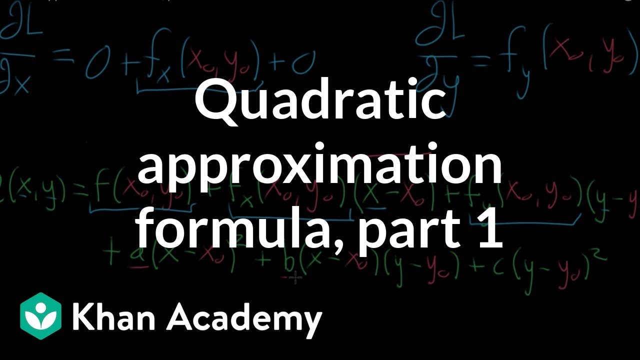
Quadratic approximation example
TLDRThis educational video delves into the concept of quadratic approximations for multivariable functions. The instructor begins by explaining the abstract form of the approximation, then provides a concrete example using the function f(x, y) = e^(x/2) * sin(y). They guide viewers through calculating the necessary partial and second partial derivatives at the point (0, π/2). The process includes evaluating the function and its derivatives at the chosen point and then plugging these values into the quadratic approximation formula. The result is a simplified polynomial that closely approximates the original function near the specified point, offering a practical tool for both computational and theoretical analysis.
Takeaways
- 📚 The script discusses quadratic approximations of multi-variable functions, focusing on the approximation of a two-variable function, f(x, y).
- 🔍 The approximation process involves breaking down the function into a constant term, linear terms, and quadratic terms to simplify the expression.
- 📈 A specific example is used to illustrate the process, with the function f(x, y) = e^(x/2) * sin(y) being approximated near the point (0, π/2).
- 🔢 The script emphasizes the importance of calculating partial and second partial derivatives to construct the quadratic approximation.
- 👨🏫 The instructor corrects a mistake regarding the coefficients of the second partial derivatives, highlighting the need for attention to detail in such calculations.
- 📝 After calculating the necessary derivatives, they are evaluated at the specified point, simplifying the approximation process.
- 📉 The quadratic approximation is then simplified by substituting the evaluated derivatives into the approximation formula, resulting in a polynomial form.
- 📊 The script mentions the practicality of using quadratic approximations for computational purposes, as polynomials are easier for computers to process.
- 📚 The approximation also serves as a theoretical tool for understanding the qualitative features of the function's graph, such as identifying saddle points.
- 📈 The script includes a visual comparison between the original function and its quadratic approximation, showing how well the approximation fits near the specified point.
- 🔮 Finally, the script previews upcoming content on a more generalizable form of writing down quadratic approximations using vector notation, applicable to functions with more than two variables.
Q & A
What is the purpose of quadratic approximations in multivariable functions?
-Quadratic approximations are used to simplify the understanding and computation of multivariable functions near a specific point. They provide a polynomial representation of the function that is easier for theoretical analysis and computational purposes.
What is the significance of the constant term in a quadratic approximation?
-The constant term in a quadratic approximation represents the value of the function at the point of approximation. It is the starting point from which the linear and quadratic terms build upon to provide a more accurate approximation.
How are linear terms identified in a quadratic approximation?
-Linear terms are identified by their structure where the variables are multiplied by constants. In the script, these terms are represented by the first partial derivatives with respect to each variable.
What does the quadratic term in a quadratic approximation represent?
-The quadratic term represents the part of the approximation that accounts for the curvature of the function. It includes terms with variables squared and cross terms, which are essential for capturing the function's behavior near the approximation point.
Why is the function f(xy) = e^(x/2) * sin(y) chosen for the example in the script?
-This function is chosen because it is relatively simple to evaluate and its derivatives are well-known, making it convenient for demonstrating the process of quadratic approximation without unnecessary complexity.
What is the role of partial derivatives in the process of quadratic approximation?
-Partial derivatives are essential in the process as they provide the coefficients for the linear and quadratic terms in the approximation. They are evaluated at the point of approximation to determine the shape and behavior of the function near that point.
Why are second partial derivatives important in the quadratic approximation?
-Second partial derivatives are crucial as they contribute to the quadratic terms of the approximation, which capture the curvature of the function. They are also used in the second partial derivative test for understanding the local behavior of the function.
What is the significance of the point (0, π/2) in the script's example?
-The point (0, π/2) is chosen as the point of approximation because it simplifies the evaluation of the function and its derivatives. At this point, the function and its derivatives have known values, which makes the example more straightforward.
How does the script correct the mistake regarding the coefficients of the second partial derivatives?
-The script corrects the mistake by acknowledging that the coefficients should be one half for each of the second partial derivatives, not one fourth as initially stated. This correction is important for the accuracy of the quadratic approximation.
What is the purpose of the graph in the script's example?
-The graph serves to visually demonstrate the accuracy of the quadratic approximation near the point of approximation. It allows viewers to see how well the polynomial approximation matches the original function's behavior in the vicinity of the chosen point.
How does the script suggest improving the quadratic approximation for more variables?
-The script suggests using vector notation to generalize the quadratic approximation for more variables. This approach simplifies the representation and computation, making it more manageable for functions with three or more variables.
Outlines
📚 Introduction to Quadratic Approximations
This paragraph introduces the concept of quadratic approximations for multi-variable functions. It discusses the complexity of the expressions involved and the intention to simplify them through a specific example. The example chosen is the function f(xy) = e^x/2 * sin(y), which is to be approximated near the point (0, π/2). The paragraph explains the need to calculate various partial and second partial derivatives of the function to facilitate the approximation process.
🔍 Calculating Partial Derivatives
The second paragraph delves into the process of calculating the necessary partial derivatives for the function f(xy). It explains the computation of the first partial derivatives with respect to x and y, and then proceeds to calculate the second partial derivatives, including the mixed partial derivative. The paragraph highlights a mistake made in the initial calculation of the second partial derivatives, which is corrected to include a factor of one half for each of them. The goal is to evaluate these derivatives at the specified point (0, π/2).
📉 Evaluating Derivatives and Approximating the Function
This paragraph focuses on evaluating the previously calculated partial derivatives at the point (0, π/2) and using these values to construct the quadratic approximation of the function. It details the process of plugging in the values into the quadratic approximation formula, correcting a previous oversight regarding the coefficients of the second partial derivatives. The paragraph simplifies the approximation to a form that highlights its polynomial nature, emphasizing the ease of computation and theoretical utility of such an approximation.
📈 Visualizing the Quadratic Approximation
The final paragraph discusses the practical and theoretical implications of the quadratic approximation. It describes the process of visualizing the original function and its quadratic approximation through graphs, noting the approximation's effectiveness near the point of interest. The paragraph also mentions the utility of quadratic approximations in theoretical analysis, such as the second partial derivative test, and hints at future discussions on more general forms of these approximations using vector notation for multi-variable functions.
Mindmap
Keywords
💡Quadratic Approximation
💡Multivariable Function
💡Partial Derivatives
💡Second Partial Derivatives
💡Mixed Partial Derivative
💡Constant Term
💡Linear Term
💡Quadratic Term
💡Taylor Expansion
💡Vector Notation
Highlights
Introduction to quadratic approximations of multi-variable functions, emphasizing the simplification of complex expressions.
Explanation of the constant term in the approximation as an evaluable numerical value.
Identification of linear terms in the approximation, highlighting their variable-times-constant nature.
Discussion of the quadratic term's significance in capturing the essence of the approximation.
Use of a specific example to demonstrate the approximation process with a multi-variable function.
Selection of a convenient point for approximation to simplify the evaluation of derivatives.
Derivation of partial derivatives necessary for the quadratic approximation.
Clarification of the process for obtaining second partial derivatives in the approximation.
Correction of a mistake regarding the coefficients of the second partial derivatives.
Evaluation of the function and its derivatives at the chosen point for approximation.
Simplification of the quadratic approximation using the evaluated constants.
Illustration of how the quadratic approximation can be used to simplify computational tasks for computers.
Theoretical implications of the quadratic approximation for understanding the shape of the graph.
Visual representation of the original function and its quadratic approximation through graphs.
Comparison of the quadratic approximation's performance near the point of approximation versus at a distance.
Introduction to the second partial derivative test and its relevance to the shape analysis of functions.
Anticipation of a future discussion on a more general form of quadratic approximation using vector notation.
Transcripts
Browse More Related Video


5.0 / 5 (0 votes)
Thanks for rating: