Quadratic approximation formula, part 2
TLDRThis video tutorial delves into the intricacies of quadratic approximation for a two-variable function 'f'. It explains the concept of 'Q', a scaffolding for approximating 'f', and how to determine the coefficients of its quadratic terms to closely match 'f's graph. The instructor emphasizes matching the second partial derivatives of 'Q' and 'f' at a point of interest, providing a step-by-step guide to compute these derivatives and equate them. The goal is to achieve a close graphical approximation, with a visual reminder that the quadratic form should mimic the function's curvature near the specified point.
Takeaways
- 📐 The script discusses the process of setting up a quadratic approximation for a two-variable function, denoted as Q(f).
- 🔍 It explains that the quadratic approximation consists of six terms, including three linear and three quadratic terms.
- 🔑 The main goal is to determine the coefficients of the quadratic terms so that Q closely approximates the function f near a specific point.
- 📈 The script emphasizes the importance of matching the second partial derivatives of Q with those of f at the point of interest.
- 🧩 It details the process of finding the first and second partial derivatives of Q with respect to both variables X and Y.
- 📝 The script provides a method to solve for the constants in the quadratic terms by equating them to the second partial derivatives of f evaluated at the point of interest.
- 📚 It mentions that for most functions, the mixed partial derivatives with respect to X and Y are equal regardless of the order of differentiation.
- 🔢 The constants a, b, and c in the quadratic terms are set to half of the respective second partial derivatives of f evaluated at the point of interest.
- 🔄 The process involves taking the first and second partial derivatives of Q with respect to X and Y, and setting them equal to the corresponding derivatives of f.
- 📉 The script uses a step-by-step approach to illustrate the computation of the second partial derivatives and how to equate them to find the constants.
- 📊 The final result is a quadratic approximation formula that includes the constants, linear, and quadratic terms, providing a close fit to the function f near the specified point.
Q & A
What is the purpose of the quadratic approximation in the context of the video?
-The purpose of the quadratic approximation is to create a function Q that closely approximates an arbitrary two-variable function f near a specific point, by matching the second partial derivatives of Q and f at that point.
What are the three main types of terms in the quadratic approximation formula presented in the video?
-The three main types of terms in the quadratic approximation formula are the constant term, the linear terms derived from the local linearization, and the quadratic terms representing the curvature of the function at the point of interest.
Why does the video mention that the quadratic approximation formula might seem more complicated than it is?
-The quadratic approximation formula might seem more complicated because it includes six different terms derived from local linearization and quadratic parts, which can make the formula appear more abstract and intricate than the underlying concept.
What does 'hugging the graph' mean in the context of the quadratic approximation?
-'Hugging the graph' refers to the quadratic approximation closely fitting the original function f near the point of interest, providing a good approximation of the function's behavior in that region.
What is the significance of matching the second partial derivatives of Q and f in the quadratic approximation process?
-Matching the second partial derivatives ensures that the curvature of the approximation Q matches that of the original function f at the point of interest, which is crucial for an accurate approximation.
Why is the mixed partial derivative important in the context of the quadratic approximation?
-The mixed partial derivative is important because it represents the rate of change of the function with respect to two variables, and matching it ensures that the approximation Q captures the correct interaction between the variables at the point of interest.
What assumption does the video make about the functions being dealt with in the context of the quadratic approximation?
-The video assumes that the functions being dealt with have the property that the order of differentiation does not affect the result, meaning that the mixed partial derivatives are equal regardless of the order in which the variables are differentiated.
How does the video suggest finding the values of the constants a, b, and c in the quadratic approximation formula?
-The video suggests setting the constants a, b, and c equal to half of the respective second partial derivatives of the original function f evaluated at the point of interest, to ensure that the second partial derivatives of the approximation Q match those of f.
What is the role of the first partial derivatives in the quadratic approximation process described in the video?
-The first partial derivatives are used to determine the linear terms in the quadratic approximation formula, which represent the first-order behavior of the function near the point of interest.
How does the video simplify the process of finding the second partial derivatives of the quadratic approximation Q?
-The video simplifies the process by breaking down the expression for Q into terms and taking the partial derivatives one term at a time, showing that the second partial derivatives of Q with respect to X and Y result in constants that can be set to match those of the original function f.
What additional resource does the video mention for further understanding of quadratic approximations?
-The video mentions an article on quadratic approximations as an additional resource for those who wish to delve deeper into the topic and practice the computations themselves.
Outlines
📚 Introduction to Quadratic Approximation
This paragraph introduces the concept of quadratic approximation for a two-variable function 'f'. The speaker sets up the scaffolding for the approximation, denoted as 'Q', which currently includes six terms. The first three terms are derived from the local linearization formula, while the latter three represent the quadratic components. The goal is to determine the coefficients for these quadratic terms to ensure that 'Q' closely follows the graph of 'f'. The speaker explains the importance of matching the second partial derivatives of 'Q' with those of 'f' at the point of interest, which includes not only the second partial derivatives with respect to each variable individually but also the mixed partial derivative, assuming the function satisfies the condition of having equal mixed partials.
🔍 Deriving Coefficients for Quadratic Terms
In this paragraph, the speaker delves into the process of finding the coefficients for the quadratic terms in the approximation formula. The focus is on calculating the second partial derivatives of 'Q' with respect to 'X' and 'Y', and ensuring they match those of the original function 'f' at the point of interest. The speaker provides a step-by-step explanation of how to compute these derivatives and match them to the function 'f'. The constants 'a', 'b', and 'c' are identified as crucial and are determined by setting them equal to half of the respective second partial derivatives of 'f' evaluated at the point of interest. The paragraph concludes with the insight that by plugging in these values, one obtains a quadratic approximation that closely fits the function 'f'. The speaker also encourages the viewer to perform these computations to solidify their understanding and refers to an article on quadratic approximations for further details.
Mindmap
Keywords
💡Quadratic Approximation
💡Scaffolding
💡Local Linearization
💡Quadratic Terms
💡Coefficients
💡Second Partial Derivatives
💡Mixed Partial Derivative
💡Point of Interest
💡Graphical Intuition
💡Constants
Highlights
Introduction of the concept of quadratic approximation for a two-variable function.
Explanation of the scaffolding for the quadratic approximation formula.
Discussion on the six different terms involved in the quadratic approximation.
Clarification that the first three terms are derived from the local linearization formula.
Description of the quadratic terms including X squared, X times Y, and Y squared.
The challenge of determining the coefficients for the quadratic terms to closely fit the function graph.
The goal of matching the second partial derivatives of Q with those of the function f.
Importance of consistency in mixed partial derivatives for most functions.
Assumption that the order of differentiation does not affect the mixed partial derivative.
Process of finding the first partial derivative with respect to X.
Derivation of the second partial derivative with respect to X to find constant 'a'.
Setting 'a' equal to one half of the second partial derivative of f with respect to X evaluated at the point of interest.
Exploration of the mixed partial derivative with respect to X and Y to find constant 'b'.
Setting 'b' equal to the mixed partial derivative of f evaluated at the point of interest.
Symmetry in the process to find constant 'c' for the second partial derivative with respect to Y.
Setting 'c' equal to one half of the second partial derivative of f with respect to Y evaluated at the point of interest.
Final quadratic approximation formula with constants a, b, and c plugged in.
Emphasis on the graphical intuition of the quadratic approximation hugging the function graph.
Encouragement for viewers to engage with the material through articles and computations.
Transcripts
Browse More Related Video
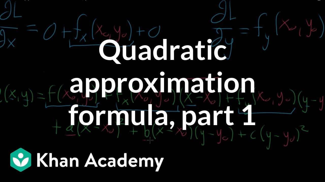
Quadratic approximation formula, part 1
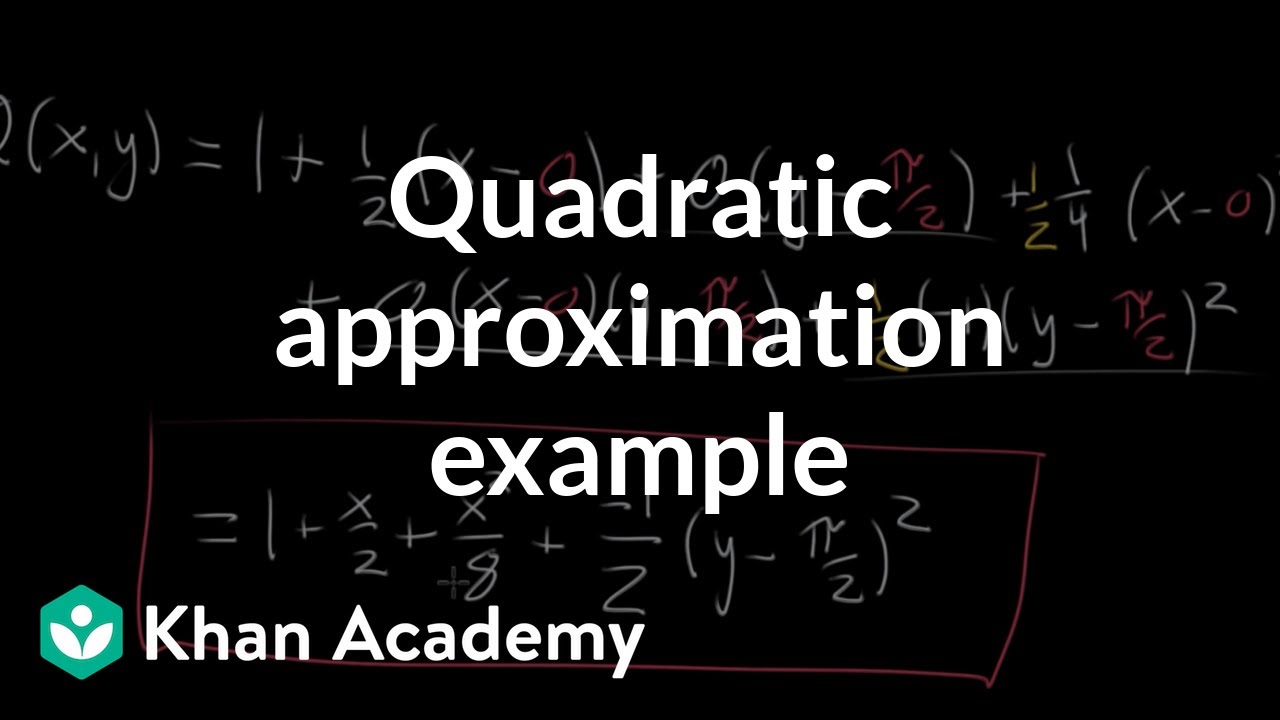
Quadratic approximation example
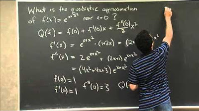
Quadratic Approximation | MIT 18.01SC Single Variable Calculus, Fall 2010
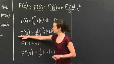
Second fundamental theorem and quadratic approximation | MIT 18.01SC Single Variable Calculus
Polynomial approximation of functions (part 1)
What do quadratic approximations look like
5.0 / 5 (0 votes)
Thanks for rating: