Math 119 Chapter 10 part 2

Brad Bolton

14 Dec 202044:31

EducationalLearning

32 Likes 10 Comments

TLDRThis script covers the fundamentals of regression analysis in a statistical context, focusing on the relationship between explanatory and response variables. It explains the construction of a regression line, the calculation of slope and y-intercept, and the application of these concepts to real-world data sets. The instructor demonstrates how to use technology to compute these values and emphasizes the importance of linear relationships in effective prediction. The summary also touches on interpreting residuals, identifying influential points, and understanding the predictive power of regression lines, concluding with advice on when to rely on regression equations versus mean values for prediction.

Takeaways

📚 The lecture covers the last part of chapter 10, focusing on building regression equations to summarize the relationship between explanatory and response variables.
📉 The regression line, represented as y hat = a + bx, is a straight line that shows how the response variable (y) changes with the explanatory variable (x).
🔍 The formulas for slope (b) and y-intercept (a) are derived from the standard deviations and correlation coefficient, emphasizing the importance of statistical understanding.
🛠️ Technology, such as calculator functions, is used to find regression values, but the formulas are still important to understand the underlying process.
📈 The instructor demonstrates using a calculator for linear regression and t-tests, showing practical steps to find the slope and y-intercept.
🧍‍♀️ An example of predicting supermodel weights from height is given, illustrating the process of using regression equations with real-world data.
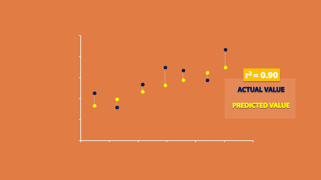
📝 The concept of residuals is introduced, explaining how they represent the difference between observed and predicted values, which is crucial for assessing the accuracy of the regression line.
📉 Residual plots are discussed as a tool to visualize the distribution of residuals and to identify patterns that might indicate a poor fit of the regression model.
🤔 The importance of distinguishing between outliers and influential points is highlighted, noting that not all outliers significantly affect the regression line.
⚖️ The script touches on the balance between using regression equations for prediction when there is a strong linear relationship and reverting to using the mean for predictions in the absence of a linear pattern.
🏁 The lecture concludes with a reminder that the regression equation is a powerful predictive tool when the data exhibits a strong linear correlation, and the course is nearing its end with upcoming exams.

Q & A

What is the main focus of the last part of chapter 10 in the script?
-The main focus is on building the regression equation, which summarizes the relationship between two variables, specifically the explanatory and response variables.
What is the formula for the regression line mentioned in the script?
-The formula for the regression line is y hat equals a plus bx, where y hat is the predicted response variable, a is the y-intercept, b is the slope, and x is the explanatory variable.
What is the purpose of the slope (b) in the regression equation?
-The slope (b) in the regression equation represents the change in the response variable (y) for a one-unit change in the explanatory variable (x).
How is the slope (b) calculated in the script?
-The slope (b) is calculated using the formula b equals r times the standard deviation of the y's divided by the standard deviation of the x's, where r is the correlation coefficient.
What is the y-intercept (a) in the regression equation and how is it found?
-The y-intercept (a) is the point where the regression line crosses the y-axis. It is calculated using the formula a equals y bar minus b times x bar, where y bar is the mean of the response variable and x bar is the mean of the explanatory variable.
What is the role of the correlation coefficient (r) in the regression analysis?
-The correlation coefficient (r) measures the strength and direction of the linear relationship between the explanatory and response variables. It is used in calculating the slope of the regression line.
How does the script differentiate between the slope (b) in the formula and the slope provided by a calculator?
-The script clarifies that there are two different b's: one in the formula for the regression line and another provided by the calculator. It emphasizes not to confuse them despite the same notation.
What is the significance of the r-squared value in the script?
-The r-squared value represents the proportion of the variance in the dependent variable that is predictable from the independent variable(s). It is a measure of how well the regression line fits the data.
How does the script use the concept of residuals in the context of regression analysis?
-Residuals are the differences between the observed values and the predicted values from the regression line. The script discusses how residuals can indicate the accuracy of the regression line and identify patterns or outliers in the data.
What is the advice given in the script for situations where the data does not fit a linear pattern?
-The script advises that if the data does not fit a linear pattern, one should use the mean for predictions instead of the regression equation, as the regression line would not be a good predictor in such cases.
How does the script handle the interpretation of the y-intercept in the context of real-world applications?
-The script explains that the y-intercept may not always make sense in real-world applications, especially when the value of the explanatory variable is zero, as in the case of predicting weight from height when height cannot be zero.

Outlines

00:00

📚 Introduction to Regression Equation

The instructor introduces the concept of building a regression equation in the context of chapter 10.3, clarifying a potential homework discrepancy with section 10.2. The purpose of the regression line is to illustrate the relationship between explanatory and response variables. The formula for the slope (b) and y-intercept (a) is discussed, emphasizing the distinction between different 'b's in various contexts. The use of technology to find these values is highlighted, with a walkthrough of using a calculator for linear regression, including finding the standard deviation and correlation coefficient (r), and applying the slope formula. The 'Old Faithful' data set is used as an example to demonstrate the process.

05:03

📉 Regression Analysis and Equation Building

This section delves deeper into regression analysis, using the example of predicting supermodel weights from their height. The process involves entering data into a calculator, plotting a linear regression, and interpreting the results, including r and r-squared values. The instructor guides through calculating the slope and y-intercept manually and verifying them with the calculator. The importance of understanding the linear relationship and building a predictive model is emphasized, concluding with the regression equation for the supermodel data.

10:07

🔍 Interpreting Regression Results and Predictions

The instructor explains how to interpret the slope and y-intercept from a regression equation, using the supermodel weight prediction as an example. The slope indicates the change in weight per inch of height, while the y-intercept, although not logically applicable in this context, is mathematically derived. The process of predicting the weight of a supermodel with a specific height is demonstrated, and the results are compared with actual data points to assess the prediction's accuracy.

15:08

📈 Studying and Test Scores: Regression Analysis

The script shifts to analyzing the relationship between study time and test scores. Data is entered into a calculator, and a regression equation is derived, including the interpretation of the slope and y-intercept. The instructor shows how to use the regression line to predict test scores based on study hours and calculates the predicted score for three hours of study. Additionally, the time required to study for a perfect test score is determined, illustrating the predictive power of the regression model.

20:12

📊 Understanding Residuals and Predictive Power

The concept of residuals is introduced as the difference between observed and predicted values. The instructor explains how residuals can indicate overprediction or underprediction and their role in assessing the regression line's accuracy. Using examples, the script demonstrates how to calculate residuals and interpret their values. The importance of small residuals for a good predictive model is highlighted, along with the signs of a bad predictor, such as large residuals or non-linear patterns.

25:13

🌡️ Temperature and Chirps: Regression Prediction

The script presents a scenario involving the relationship between temperature and the number of chirps per second in crickets. Given a regression equation and a Pearson correlation coefficient, the instructor discusses the predictability of chirps based on temperature. The process of predicting chirps for a specific temperature and calculating residuals for observed data is shown, reinforcing the use of regression for prediction when a strong linear relationship exists.

30:14

🚗 Car Mileage Prediction Using Regression

The final part of the script discusses predicting a car's highway mileage based on city mileage, using a provided regression equation. The slope and y-intercept are interpreted, explaining how an increase in city miles per gallon affects highway miles per gallon. The predicted highway mileage for a car with a specific city mileage is calculated, and the residual is determined using actual versus predicted values. The script concludes with calculating the proportion of variation in highway mileage explained by city mileage, emphasizing the predictive strength of the model.

35:17

📝 Conclusion and Final Thoughts on Regression

In the concluding paragraph, the instructor summarizes the key points of regression analysis covered in chapter 10. The importance of a strong linear correlation for effective predictions using a regression equation is reiterated. The instructor advises using the mean for predictions when data does not exhibit a linear pattern, highlighting the limitations of regression in such cases. The script ends with a reminder to prepare for upcoming exams, signaling the completion of the course material on regression.

Mindmap

Keywords

💡Regression Equation

A regression equation is a mathematical formula that describes the relationship between two variables, typically an explanatory variable (x) and a response variable (y). In the context of the video, the regression equation is used to predict the value of the response variable based on the explanatory variable. For example, the script discusses building a regression equation to predict supermodel weights from their height, where height is the explanatory variable and weight is the response variable.

💡Explanatory and Response Variables

In statistics, explanatory variables are those thought to influence the response variable. The response variable is the outcome or result being predicted or explained. The video emphasizes the importance of identifying these variables correctly to build an accurate regression model. For instance, in predicting weights from heights, height is the explanatory variable, and weight is the response variable.

💡Linear Relationship

A linear relationship implies that there is a straight-line connection between two variables, which can be described by a linear equation. The video's theme revolves around identifying whether a linear relationship exists between variables and then using that relationship to predict outcomes. The script mentions that the regression line helps to determine if there is a linear relationship between studying time and test scores.

💡Slope

The slope of a line in a regression equation represents the rate of change of the response variable for a one-unit change in the explanatory variable. It is a crucial component of the regression equation and indicates the direction and steepness of the relationship. The script uses the slope to interpret how changes in the explanatory variable, such as height or study hours, affect the response variable, like weight or test scores.

💡Y-Intercept

The y-intercept is the point where the regression line crosses the y-axis. It represents the predicted value of the response variable when the explanatory variable is zero. In the video, the y-intercept is discussed in the context of the regression equation, and its interpretation varies depending on the specific scenario, such as predicting weights at a height of zero.

💡Residuals

Residuals are the differences between the observed values and the values predicted by the regression line. They measure the accuracy of the regression model. The script explains how to calculate residuals and interpret their meaning, such as indicating overprediction or underprediction by the regression line.

💡R-Squared

R-squared is a statistical measure that represents the proportion of the variance for the dependent variable that's explained by the independent variables in a regression model. The video uses r-squared to explain the proportion of variation in one variable that can be accounted for by another, such as the relationship between city and highway miles per gallon.

💡Correlation Coefficient (R)

The correlation coefficient, often denoted as 'r', is a statistical measure that expresses the extent to which two variables are linearly related. The closer the absolute value of 'r' is to 1, the stronger the linear relationship. The script discusses using 'r' to determine the strength of the linear relationship between variables, such as city mileage and highway mileage.

💡Outliers

Outliers are data points that differ significantly from other observations. They can sometimes skew the results of an analysis. The video mentions outliers in the context of regression analysis, noting that while not all outliers are influential points, all influential points are outliers, which can affect the regression line's accuracy.

💡Predictive Power

Predictive power refers to the ability of a regression model to accurately predict outcomes based on the relationship between variables. The script discusses the features of a regression line that indicate good predictive power, such as small residuals and the absence of non-linear patterns, which suggest that the model is a reliable predictor of the response variable.

Highlights

Introduction to building a regression equation in Chapter 10, focusing on the relationship between explanatory and response variables.

Explanation of the regression line formula, y hat equals a plus bx, and the distinction between the y-intercept (a) and the slope (b).

Clarification on the difference between the 'b' in the formula and the 'b' used by calculators.

Demonstration of using technology to find regression values instead of manual calculation.

Procedure for inputting data into a calculator for two-variable statistical analysis.

Calculation of the slope (b) using the standard deviation and correlation coefficient.

Illustration of finding the y-intercept (a) using the mean values of x and y.

Application of the regression equation to predict supermodel weights based on height.

Interpretation of the slope in the context of height and weight, and the meaning of the y-intercept.

Use of a calculator to find the predicted weight of a supermodel with a specific height.

Introduction to the concept of residuals and their role in evaluating the accuracy of predictions.

Discussion on how to identify influential points and outliers in a scatter plot.

Explanation of how to calculate and interpret residuals for predicting systolic blood pressure.

Use of regression analysis to predict test scores based on study time and interpretation of results.

Method to determine the study time required to achieve a specific test score using regression.

Analysis of the relationship between car city mileage and highway mileage using regression.

Interpretation of the regression line's slope and y-intercept for predicting highway mileage.

Calculation of the predicted highway mileage for a car with a given city mileage.

Determination of residuals to evaluate the prediction accuracy of highway mileage.

Explanation of r-squared and its significance in explaining the variation in dependent variables.

Guidance on when to use the mean for predictions instead of a regression equation due to weak linear relationships.

Transcripts

Browse More Related Video

Linear regression using R programming

Regression and R-Squared (2.2)

10.2.1 Regression - Essential Terminology and Background Related to Regression

Elementary Stats Lesson #5

Calculating Residuals & Making Residual Plots on TI-84 Plus

RESIDUALS! What are they? how to find them, how to use them

Related Tags

Linear Regression Predictive Modeling Data Analysis Statistical Methods Correlation Coefficient Residual Analysis Regression Equation Predictive Power Calculator Usage Educational Content