22. Finding Natural Frequencies & Mode Shapes of a 2 DOF System
TLDRIn this MIT OpenCourseWare lecture, Professor Dave Gossard explores multiple degree of freedom systems, focusing on their natural frequencies and modes. Using a two-spring, two-mass system as an example, he demonstrates the concept of eigenvalues and eigenvectors, showing how systems can oscillate at different frequencies with distinct amplitudes. Gossard simplifies the algebra with a special case of identical masses and springs, deriving the characteristic equation to find natural frequencies. He also discusses the importance of understanding damping types, such as Coulomb damping, and concludes with a practical demonstration using a mechanical apparatus to illustrate the theoretical concepts.
Takeaways
- 📚 The lecture introduces the concept of multiple degree of freedom systems, which are generalizations of single degree of freedom systems with multiple natural frequencies and eigenvalues.
- 🔍 The demonstration involves a physical system with two springs and two masses, illustrating the principles discussed in the lecture.
- 📐 Displacements in the system are defined with respect to the static equilibrium position, a concept previously covered by Professor Vandiver.
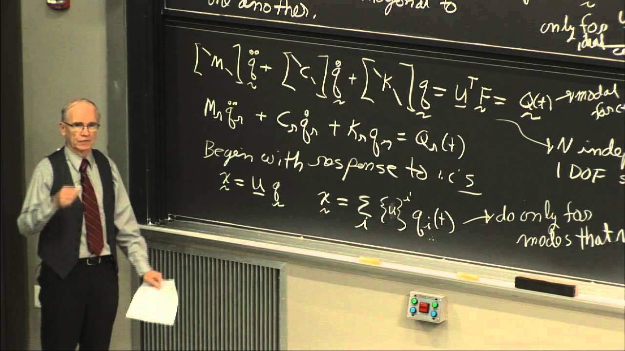
- 📈 The equations of motion for the system can be derived using free body diagrams or Lagrangian mechanics, resulting in a matrix form that simplifies the analysis.
- 🧠 Matrix notation is emphasized for handling multiple degrees of freedom due to its efficiency in dealing with repetitive calculations.
- 🎓 The special case of identical masses and springs simplifies the equations, making it easier to find the natural frequencies and modes of the system.
- 🌀 Harmonic motion is assumed for the analysis, where masses oscillate at the same frequency but with different amplitudes.
- 🔢 The characteristic equation, derived from the determinant of the system matrix, provides the natural frequencies of the system.
- 📉 The natural modes, or eigenvectors, represent the amplitude ratios of the system's oscillations at its natural frequencies.
- 🤔 The lecture includes interactive problem-solving with the audience, emphasizing the importance of understanding the underlying physics and mathematics.
- 📊 MATLAB is used to simulate the system's behavior, demonstrating how initial conditions affect the oscillation frequencies and amplitudes.
Q & A
What is the main topic of the lecture?
-The main topic of the lecture is multiple degree of freedom systems, focusing on the generalization of concepts such as equations of motion, natural frequencies, and the introduction of natural modes or eigenvectors.
Why does the professor mention MIT OpenCourseWare at the beginning?
-The professor mentions MIT OpenCourseWare to encourage donations and to inform the audience about the availability of additional materials from hundreds of MIT courses on their website, ocw.mit.edu.
What is the significance of Professor Vandiver being out of town?
-Professor Vandiver being out of town is significant because it indicates that Dave Gossard is substituting for him and conducting the lecture for the day.
How does the professor describe the physical system used for demonstration in the lecture?
-The professor describes the physical system as a classic textbook case of two springs and two masses, with the displacements indicated as X1 and X2, and the system is defined with respect to the static equilibrium position.
What is the method used to derive the equations of motion for the two-spring, two-mass system?
-The equations of motion for the two-spring, two-mass system can be derived either by the direct method, which involves creating free body diagrams and applying the sum of forces in the x direction for each mass, or by using Lagrange's method, which involves creating expressions for kinetic and potential energy and applying Lagrange's equations.
Why does the professor prefer matrix notation for multiple degrees of freedom systems?
-The professor prefers matrix notation for multiple degrees of freedom systems because it simplifies the repetitive nature of the equations and makes it easier to handle the algebra involved in these systems.
What is the special case considered by the professor to simplify the algebra?
-The special case considered by the professor is when the masses (M1 and M2) are identical and can be simply called M, and the springs (K1 and K2) are also identical, simply called K, which simplifies the equations of motion.
What is the term used for the characteristic equation derived from the determinant of the system matrix?
-The characteristic equation is derived from the determinant of the system matrix and is used to find the natural frequencies (omega) of the system.
How does the professor explain the concept of natural modes or eigenvectors?
-The professor explains natural modes or eigenvectors as the relative amplitudes or magnitudes of the oscillations of the masses in a multiple degree of freedom system, which are associated with each natural frequency.
What is the purpose of the MATLAB simulation shown by the professor?
-The purpose of the MATLAB simulation is to demonstrate the behavior of the two-spring, two-mass system with different initial conditions, illustrating how the system oscillates at different natural frequencies and amplitudes based on those conditions.
What is the physical demonstration used to validate the theory discussed in the lecture?
-The physical demonstration involves a real system made by Professor Vandiver's machinist, which is a second-order system with a steel rod, sliding masses, and springs. The demonstration aims to validate the theory by showing the system's behavior in response to different conditions.
How does the professor address the issue of damping in the physical demonstration?
-The professor addresses the issue of damping by identifying it as Coulomb damping, which is a type of friction that causes the system to slow down and eventually stop. This is different from viscous damping, which generates a force proportional to the velocity.
What is the method used by the professor to estimate the masses of the system in the physical demonstration?
-The professor estimates the masses by taking measurements of the diameters and lengths of the cylindrical masses and using the density of brass to calculate their masses.
How does the professor determine the spring constants (K1 and K2) for the physical demonstration?
-The professor determines the spring constants by first measuring the period of oscillation for one mass with both springs and then for the other mass with only one spring. By comparing these measurements, he calculates the spring constants.
What is the significance of the initial conditions set by the professor in the physical demonstration?
-The initial conditions set by the professor are meant to excite specific natural modes of the system, allowing for the observation of the system oscillating at its natural frequencies with distinct amplitudes and directions.
How does the professor validate the identified system parameters and the theory?
-The professor validates the identified system parameters and the theory by comparing the observed natural modes and frequencies from the physical demonstration with those predicted by the computational procedure using the identified parameters.
Outlines
📚 Introduction to Multiple Degree of Freedom Systems
The lecture begins with an introduction to multiple degree of freedom systems, a topic that expands upon the single degree of freedom systems previously studied. Dave Gossard, substituting for Professor Vandiver, sets the stage for the day's lecture, which includes both theoretical concepts and a physical demonstration. The importance of understanding multiple degrees of freedom is emphasized, as these systems possess multiple natural frequencies and eigenvalues, key concepts that will be elaborated upon throughout the lecture.
🔍 Exploring System Dynamics with Matrix Notation
This paragraph delves into the dynamics of systems with multiple degrees of freedom, using matrix notation as a preferred method for handling the equations of motion. The transition from direct methods or Lagrange's equations to matrix form is discussed, highlighting the simplicity and elegance of matrix algebra in solving for system dynamics. The example of a two-spring, two-mass system is used to illustrate the process, with the equations of motion being rearranged into a matrix form for easier analysis.
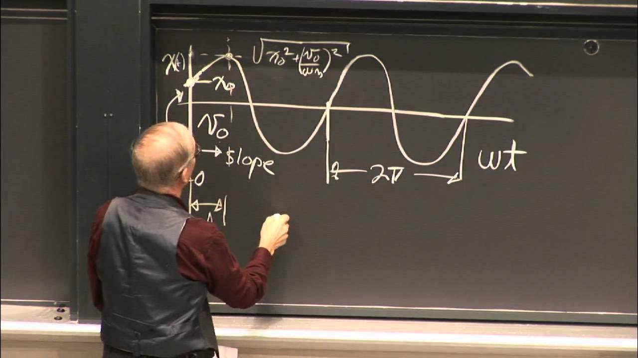
📐 Harmonic Motion and the Simplification of Equations
The concept of harmonic motion is introduced, where it is assumed that the masses oscillate at the same frequency but with different amplitudes. This assumption simplifies the equations of motion, allowing for a clearer understanding of the system's behavior. The process of differentiating the harmonic motion equations and substituting them back into the equations of motion is explained, leading to a set of linear equations that can be solved for the amplitude ratios.
🧩 Solving for Natural Frequencies and Amplitudes
The lecture continues with the solution of the characteristic equation, derived from the determinant of the system's matrix form, to find the natural frequencies (ω) of the system. The natural frequencies are identified as the eigenvalues of the system. The process of finding the amplitude ratios (A1/A2) for the system's natural modes is also discussed, emphasizing the relationship between these amplitudes and the system parameters.
📉 Understanding Natural Modes and System Response
The notion of natural modes, or eigenvectors, is introduced as a key characteristic of multiple degree of freedom systems. These modes describe the system's response to initial conditions and are unique to each natural frequency. The lecture explains how the system can be thought of as decoupled into independent subsystems, each oscillating at its own natural frequency with a distinct amplitude ratio.
🤔 Interactive Learning: MATLAB Simulations and Real-World Applications
The use of MATLAB as a tool for simulating and visualizing the behavior of multiple degree of freedom systems is demonstrated. The professor discusses the program's capabilities and limitations, highlighting its power for matrix operations and differential equation solving. The simulation of a two-spring, two-mass system with specific initial conditions is shown, illustrating how the system oscillates at a particular natural frequency with distinct amplitudes for each mass.
🔧 Practical Application: Estimating System Parameters
The lecture shifts towards a practical application, where the professor discusses the challenges of determining the parameters of a real-world system, such as masses and spring constants, without disassembling it. The audience is engaged in a brainstorming session to find creative solutions to estimate these parameters, emphasizing the engineering aspect of the problem.
🔬 Experimental Determination of Spring Constants
The paragraph describes an experimental approach to determine the spring constants of a physical system. By freezing one mass and displacing the other, the natural frequency associated with one spring and the mass can be measured. This frequency, along with the measured period, allows for the calculation of the spring constant (K2) using the formula for an undamped harmonic oscillator.
📊 Verification of Theoretical Predictions with Physical Demonstration
The lecture concludes with a physical demonstration that verifies the theoretical predictions made earlier. Using a custom-made device to set initial conditions, the professor demonstrates the first and second natural modes of the system, showing that the theoretical calculations match the observed behavior. This practical validation of the theory reinforces the understanding of multiple degree of freedom systems.
📈 Final Thoughts and Thanksgiving Wishes
In the final paragraph, the professor wraps up the lecture by summarizing the key findings and emphasizing the successful application of theoretical knowledge to a real-world system. The lecture concludes with well-wishes for the upcoming Thanksgiving holiday, highlighting the integration of education with social customs.
Mindmap
Keywords
💡Multiple Degree of Freedom Systems
💡Natural Frequencies
💡Eigenvalues
💡Eigenvectors
💡Equations of Motion
💡Matrix Notation
💡Characteristic Equation
💡Harmonic Motion
💡Amplitude Ratios
💡MATLAB
💡Coulomb Damping
Highlights
Introduction to multiple degree of freedom systems, a generalization from single degree of freedom systems.
Explanation of systems with multiple degrees of freedom having multiple natural frequencies, also known as eigenvalues.
Introduction to the concept of natural modes or eigenvectors in the context of multiple degree of freedom systems.
Use of matrix notation for the equations of motion in multiple degree of freedom systems for simplicity and repetitive quality.
Demonstration of the two-spring, two-masses system as a classic textbook case for illustrating multiple degree of freedom systems.
Discussion on the displacements being defined with respect to the static equilibrium position in mechanical systems.
Illustration of deriving equations of motion using both the direct method and Lagrange's equation, resulting in the same outcome.
Special case analysis with identical masses and springs to simplify the algebra involved in the system's equations.
Assumption of harmonic motion where masses oscillate at the same frequency but differ in magnitudes.
Derivation and explanation of the characteristic equation for finding the natural frequencies of the system.
Calculation of the system's natural frequencies using the quadratic formula applied to the characteristic equation.
Introduction and explanation of the concept of natural modes in relation to amplitude ratios and eigenvalues.
Demonstration of MATLAB programming for simulating the behavior of multiple degree of freedom systems.
Use of initial conditions to observe the system oscillating at specific natural frequencies corresponding to natural modes.
Discussion on the arbitrary and complex response of multiple degree of freedom systems to general initial conditions.
Practical demonstration of a real-world second-order system with a steel rod and masses to illustrate theoretical concepts.
Identification of damping in the real-world system, specifically Coulomb damping due to friction.
Comparison between the theoretical models and the behavior of the actual mechanical system during the demonstration.
Challenge of identifying system parameters such as masses and spring constants in a real-world scenario without disassembling the apparatus.
Innovative approach to estimate masses using measurements and material density to feed into computational models.
Method to determine spring constants by freezing one mass and measuring the natural frequency of the other in a damped system.
Validation of theoretical models through practical demonstrations and adjustments to match the observed natural frequencies.
Final demonstration of the mechanical system oscillating in its natural modes, confirming the accuracy of the identified parameters and theoretical predictions.
Transcripts


5.0 / 5 (0 votes)
Thanks for rating: