What does the Laplace Transform really tell us? A visual explanation (plus applications)
TLDRThis video explores the Laplace transform's role in analyzing oscillatory systems like a mass on a spring, contrasting it with the Fourier transform. It explains how the Laplace transform reveals sinusoids and exponentials in a function, turning calculus into algebra by simplifying differential equations into solvable algebraic forms. The video demonstrates how poles and zeros in the Laplace domain indicate a system's behavior, crucial for control systems design. It also promotes Brilliant's courses on differential equations and other advanced topics, offering a hands-on learning approach with exercises and animations.
Takeaways
- 😀 The video discusses different types of motion a mass on a spring can exhibit, such as sinusoidal motion, exponential decay, a combination of both, and other non-ideal conditions.
- 🔍 The Laplace transform is introduced as a tool that can reveal both sinusoids and exponentials present in a function, contrasting with the Fourier transform which focuses on sinusoids.
- 📚 The script explains that the Fourier transform outputs a function of Omega, indicating the presence of sinusoids in a signal, and is visualized with spikes representing frequencies.
- 📉 The y-intercept of the Fourier transform corresponds to the area under the curve of the original function, which is an important property for understanding the signal's total contribution.
- 🔧 The Laplace transform is shown to be an extension of the Fourier transform, incorporating exponential decay through the use of the complex variable 's', which is α + iω.
- 📈 The video illustrates how the Laplace transform can be visualized in a 3D plot, with the real and imaginary components of 's' on the x and y axes, and the magnitude of the output on the z-axis.
- 🎛️ The script explains that the Laplace transform simplifies the analysis of systems, such as a mass on a spring, by transforming differential equations into algebraic equations.
- 📊 The concept of poles and zeros in the context of the Laplace transform is introduced, which are critical for understanding the behavior of the system's response.
- 🔧 The video demonstrates how the Laplace transform can be used to solve for the output of a system given an input, by analyzing the locations of the poles and zeros.
- 🛠️ The script concludes by emphasizing the utility of the Laplace transform in control systems, where it allows for the design and analysis of system responses to various inputs.
- 📚 The video encourages further learning on the topic through Brilliant's courses on differential equations and other advanced mathematical concepts.
Q & A
What are the four possible outcomes when a mass on a spring system is released?
-The four outcomes are: 1) Completely sinusoidal motion with no damping, 2) Exponential decay in a viscous fluid, 3) A combination of oscillation and decay with weaker damping or stronger spring, and 4) Any other behavior due to input forces or non-ideal conditions.
What does the Laplace transform visually tell us about a function?
-The Laplace transform visually tells us which sinusoids and exponentials are present in a function, essentially providing a way to analyze both the frequency and decay components.
How is the Fourier transform related to the Laplace transform?
-The Fourier transform is essentially a slice of the Laplace transform, obtained when the real part of 's' in the Laplace transform (α) is set to zero, leaving only the imaginary part (iω).
What does the y-intercept of the Fourier transform represent?
-The y-intercept of the Fourier transform represents the area under the curve of the original function, which is the output when ω equals zero.
How does the presence of damping affect the motion of a mass on a spring?
-Damping affects the motion by introducing a force that is a multiple of velocity, which can lead to exponential decay or a combination of oscillation and decay, depending on the strength of the damping and the spring.
What is the significance of the poles in the context of the Laplace transform?
-Poles in the Laplace transform represent the values of 's' for which the denominator of the Laplace transform becomes zero, indicating points where the system's response becomes unbounded or where the system's behavior changes significantly.
How does the Laplace transform simplify the process of solving differential equations?
-The Laplace transform simplifies solving differential equations by converting them into algebraic equations in the 's' domain, making it easier to manipulate and solve, especially for control systems analysis.
What is the role of the exponential term e^(-αt) in the Laplace transform?
-The exponential term e^(-αt) in the Laplace transform allows for the analysis of the decay or growth of the function over time, and it is crucial for capturing the transient behavior of the system.
How does the Laplace transform handle non-zero initial conditions in a differential equation?
-The Laplace transform accounts for non-zero initial conditions by including additional terms related to these conditions when transforming the derivatives of the function.
What is the purpose of the Brilliant platform mentioned in the video?
-Brilliant is an educational platform that offers courses on various subjects, including differential equations. It provides hands-on exercises, intuitive animations, and in-depth explanations to help users grasp concepts from basics to advanced levels.
Outlines
🌀 Introduction to Oscillation and Laplace Transform
The video, sponsored by Brilliant, begins with an exploration of a mass-spring system and its potential behaviors, such as sinusoidal motion, exponential decay, or a combination of both. It introduces the concept of damping force and its effect on oscillation. The Laplace transform is then explained as a tool to analyze both sinusoids and exponentials in a function, contrasting it with the Fourier transform, which only accounts for sinusoids. The Fourier transform is shown to be a slice of the Laplace transform, with the latter providing a more comprehensive view of a function's components. The video also demonstrates how to apply the Fourier transform to a function with both sinusoidal and exponential elements, illustrating the process of obtaining the magnitude plot for different frequencies.
📚 Laplace Transform vs. Fourier Transform
This section delves deeper into the relationship between the Laplace transform and the Fourier transform. The Laplace transform is shown to be an extension of the Fourier transform, incorporating an additional 's' parameter, which represents a complex number α + iω. The video explains that the Laplace transform can be visualized as a 3D plot, with the Fourier transform existing as a 2D slice along the imaginary axis (α=0). The process of constructing the Laplace transform by varying α and plotting the Fourier transform of the function multiplied by e^(-αt) is described. The video also highlights the importance of the region of convergence in the Laplace transform, where the function converges to zero, and demonstrates how the Laplace transform can represent different behaviors of a system depending on the pole locations.
🔍 Analyzing System Dynamics with Laplace Transform
The video script explains how the Laplace transform can be used to analyze and solve differential equations that describe physical systems, such as a mass on a spring. By taking the Laplace transform of both sides of a differential equation, the complex calculus problem is transformed into a simpler algebraic one. The script uses an example of a mass-spring system under a constant force to illustrate this process. It shows how the Laplace transform can reveal the system's behavior through the analysis of poles and zeros in the complex plane. The video also discusses how changing parameters like the spring constant or damping coefficient affects the system's response, as indicated by the movement of poles on the complex plane.
🛠️ Laplace Transform in Control Systems and Engineering
This part of the script focuses on the practical applications of the Laplace transform in control systems and engineering. It emphasizes the transform's ability to simplify the solving of differential equations by converting them into algebraic expressions. The video uses a mass-spring-damper system as an example to demonstrate how the Laplace transform can be used to find the system's response to various inputs. It also touches on the concept of pole-zero plots and how they can be used to understand and design system behavior. The script concludes by highlighting the educational resources available on Brilliant for further learning in differential equations and related advanced topics.
👋 Conclusion and Call to Action
The final paragraph wraps up the video with a call to action for the viewers. It encourages them to like and subscribe for more content, and provides information on how to access additional learning resources through Brilliant. The video creator promotes Brilliant's courses on differential equations and other advanced topics, offering a discount for an annual premium subscription. The paragraph ends with a reminder of the educational value provided by the platform and an invitation for viewers to engage with the content and the community.
Mindmap
Keywords
💡Sinusoidal Motion
💡Exponential Decay
💡Damping
💡Laplace Transform
💡Fourier Transform
💡Complex Numbers
💡Magnitude
💡Poles
💡Differential Equations
💡Control Systems
Highlights
The video discusses four possible outcomes of a mass on a spring system: sinusoidal motion, exponential decay, a combination of both, and other non-ideal conditions.
The Laplace transform is introduced as a method to analyze functions containing both sinusoids and exponentials, while the Fourier transform focuses on sinusoids.
The Fourier transform is shown to be a subset of the Laplace transform, with the Fourier transform represented as a slice of the Laplace transform at α=0.
The process of applying the Fourier transform to a function is demonstrated, illustrating how it decomposes a function into its constituent sinusoids.
The significance of the y-intercept of the Fourier transform is explained as the area under the curve of the original function.
A complex function involving both sinusoidal and exponential components is transformed using the Fourier transform.
The concept of magnitude in the Fourier transform is introduced, showing how to plot the magnitude against the input frequency.
The Laplace transform formula is presented, highlighting its similarity to the Fourier transform but with the addition of an exponential term.
A detailed explanation of how the Laplace transform extends the Fourier transform by including exponential decay is provided.
The Laplace transform is visualized in four dimensions, with the real and imaginary components of both the input and output.
The video demonstrates how the Laplace transform can be used to analyze the transient response of a system from the time it turns on.
The relationship between the poles and zeros of a function in the Laplace domain and the original time-domain function is explored.
The concept of the region of convergence in the Laplace transform is introduced, explaining where the transform exists.
The video explains how the Laplace transform helps in solving differential equations by converting them into algebraic equations.
An example of solving a mass-spring-damper system using the Laplace transform is provided, illustrating its practical application.
The impact of changing system parameters like spring constant and damping on the pole-zero plot and system response is discussed.
The video concludes by emphasizing the importance of the Laplace transform in control systems analysis and design.
Brilliant.org is promoted as a resource for further learning on differential equations and related advanced topics.
Transcripts
Browse More Related Video

Physics Students Need to Know These 5 Methods for Differential Equations
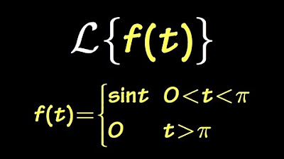
Laplace transform of a piecewise function, sect7.2#11
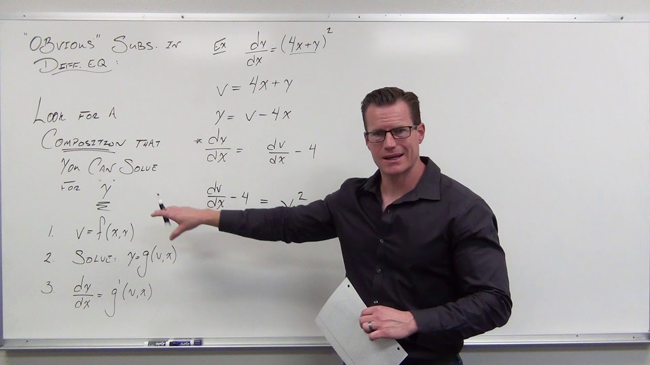
Solving Differential Equations with a Composition (Obvious) Substitution (Differential Equations 22)
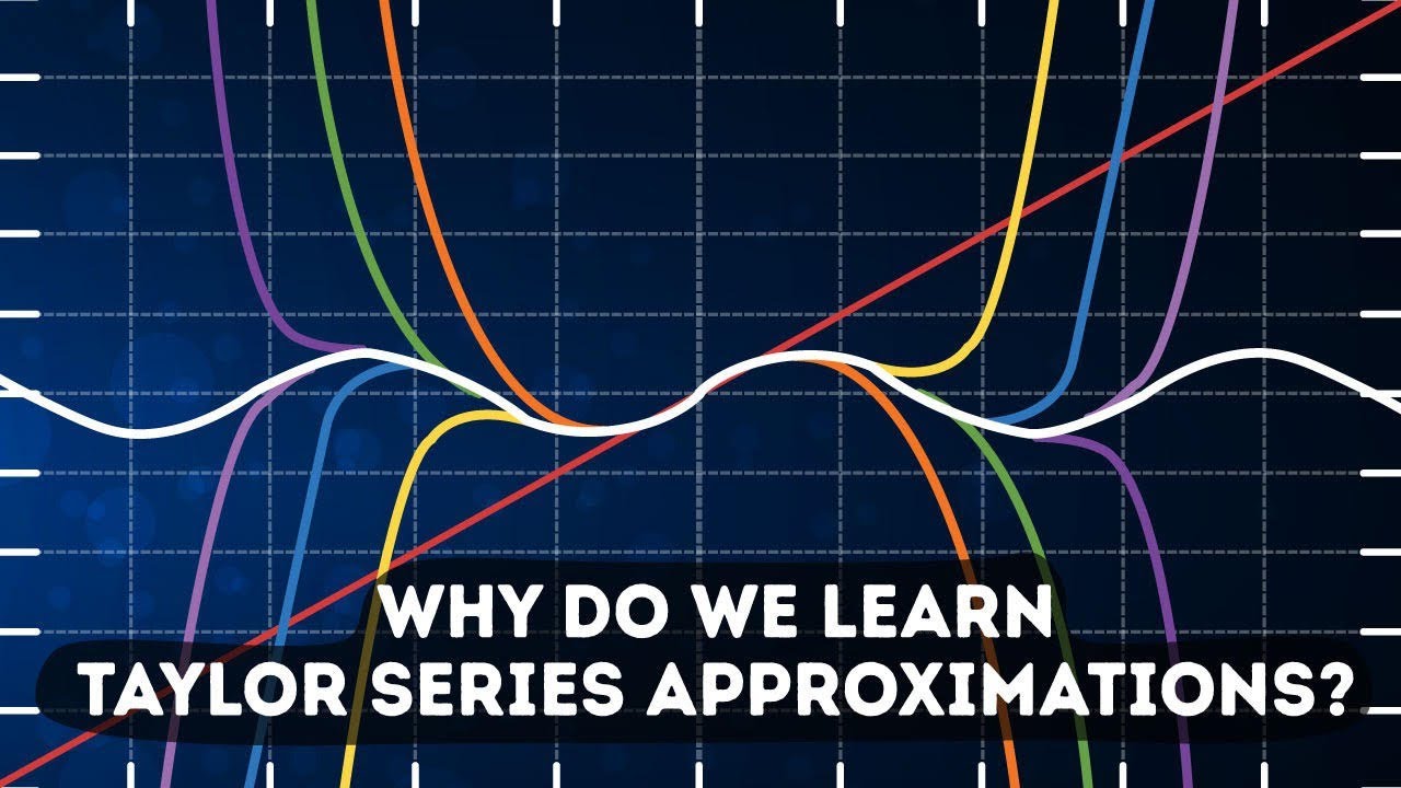
Dear Calculus 2 Students, This is why you're learning Taylor Series
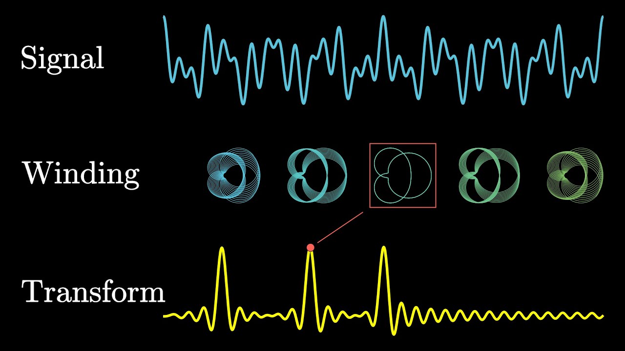
But what is the Fourier Transform? A visual introduction.
This is why you're learning differential equations
5.0 / 5 (0 votes)
Thanks for rating: