Lagrange Multipliers | Geometric Meaning & Full Example
TLDRThis video explores the application of calculus in optimization with constraints, focusing on finding maximums and minimums of functions within a restricted domain. The presenter introduces the concept of Lagrange multipliers, a method for determining the extrema of a function subject to a constraint, using the example of a function restricted to a circle. The video explains the geometric interpretation of the method, where the gradients of the function and constraint are proportional, and provides an algebraic approach to solving for the critical points. It concludes with a practical example, solving for the maximum and minimum values of the given function on the circle, and encourages viewers to engage with the content and explore further videos on multivariable calculus.
Takeaways
- 📚 The script discusses the concept of optimization in calculus, specifically focusing on finding maximums and minimums of functions under constraints.
- 📈 It introduces a function f(x, y) = x^2 - y^2 + 1, which has a saddle point at (0, 0) but extends infinitely in some directions and approaches negative infinity in others.
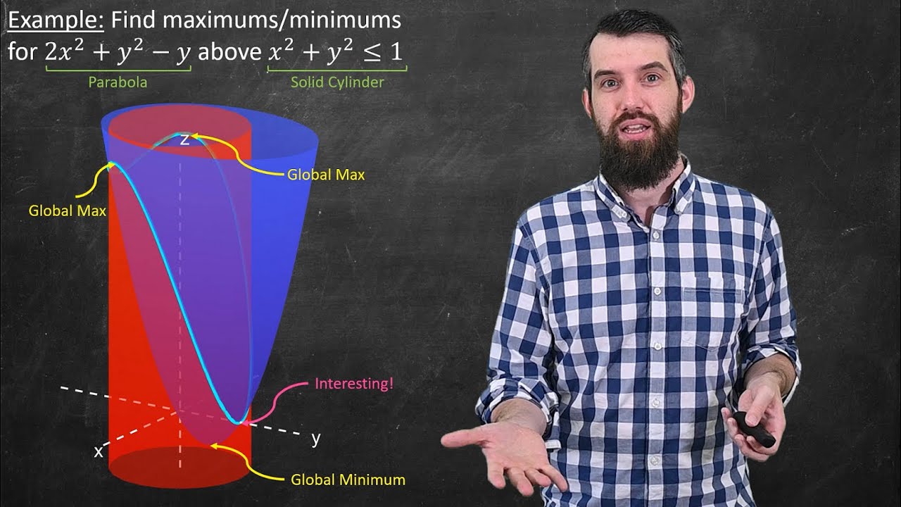
- 🔵 The video uses a graphical example involving a circle (x^2 + y^2 = 1) as a constraint to find the maximum and minimum values of the function within this domain.
- 📊 The concept of level curves is explained, which represent constant values of the function and help visualize the function's behavior relative to the constraint.
- 🔍 The script highlights the importance of the level curve that just touches the constraint, as it is a candidate for the maximum or minimum of the function under the constraint.
- 📐 The method of Lagrange multipliers is introduced as a mathematical approach to find these extrema under constraints.
- 🔢 The video explains that the gradients of the function and the constraint must be scalar multiples of each other at the points of extremum, leading to a system of equations involving the function, constraint, and a multiplier λ.
- 🧩 The script provides a step-by-step algebraic solution using the function's gradient, the constraint's gradient, and the relationship between them to find potential extremum points.
- 🔄 It is noted that solving these equations gives multiple points, but not all may satisfy the constraint or represent actual maximums or minimums.
- 📝 The video concludes by emphasizing the need to evaluate the function at the candidate points to determine which are true maximums or minimums.
- 🔗 The script invites viewers to explore more on the topic through a playlist of multivariable calculus videos, suggesting further learning opportunities.
Q & A
What is one of the most powerful applications of calculus mentioned in the video?
-One of the most powerful applications of calculus mentioned is optimization, specifically finding the maximum or minimum values of a function under certain constraints.
What is a special type of optimization discussed in the video?
-The special type of optimization discussed is when you are asked to find the maximum or minimum of a function but with a given constraint or restriction, such as being on a particular curve.
What is the function given in the video as an example?
-The function given as an example in the video is f(x, y) = x * y + 1.
What is the constraint used in the example to restrict the function?
-The constraint used in the example is a circle defined by the equation x^2 + y^2 = 1.
What method is introduced in the video to find the maximums and minimums of functions under constraints?
-The method introduced in the video is called the Lagrange multipliers, which provides a way to determine the maximums and minimums of functions under given constraints.
How does the video explain the relationship between the level curves and the constraint curve?
-The video explains that one of the level curves barely touches the constraint curve at a point, indicating a potential maximum or minimum. The tangent lines of both the level curve and the constraint curve at this point are the same, suggesting that the gradients are scalar multiples of each other.
What geometric property is used in the Lagrange multiplier method to relate the gradients of the function and the constraint?
-The geometric property used is that the gradients of the function and the constraint are normal to the same tangent line at the point of contact, meaning they are scalar multiples of each other.
What are the equations used in the Lagrange multiplier method to find the maximums and minimums?
-The equations used are the scalar multiple relationship between the gradients of the function and the constraint, and the original constraint equation itself, such as G(x, y) = 0.
How does the video illustrate the process of finding the maximum and minimum points on the constraint curve?
-The video illustrates this by solving the system of equations derived from the gradients and the constraint, and then evaluating the function at the points obtained to determine which are the maximums and minimums.
What is the significance of the level curve that just barely touches the constraint curve?
-The level curve that just barely touches the constraint curve is significant because it represents the candidate for the maximum or minimum of the function on the constraint curve.
How does the video use the concept of gradients to solve for the points of maximum and minimum?
-The video uses the concept of gradients to establish a relationship between the gradient of the function and the gradient of the constraint, setting them as scalar multiples of each other, and then solving the resulting system of equations to find the points of maximum and minimum.
Outlines
📚 Introduction to Constrained Optimization with Calculus
This paragraph introduces the concept of optimization in calculus, specifically focusing on finding maximums and minimums of functions under given constraints. The video aims to explore a special case of optimization where constraints are defined, such as finding the maximum or minimum of a function restricted to a particular curve, illustrated with a graph of a function with a saddle point and a constraint represented by a circle. The method of Lagrange multipliers is introduced as a tool to solve such optimization problems, with an example of a function and its level curves in the context of the constraint curve.
🔍 Geometric Interpretation and Algebraic Formulation of Lagrange Multipliers
The second paragraph delves deeper into the geometric interpretation of the Lagrange multipliers method, explaining how the gradient of the function and the gradient of the constraint are related when the function's level curve just touches the constraint curve. It discusses the algebraic formulation of the method, involving the gradients of the function and constraint being scalar multiples of each other and the original constraint equation. The paragraph provides an example with a specific function and constraint, deriving the equations that need to be solved to find the points of maximum and minimum values under the constraint.
📉 Solving the Optimization Problem and Identifying Extremes
The final paragraph concludes the video script by solving the optimization problem using the derived equations from the previous paragraph. It describes the process of finding the points where the function's level curves intersect with the constraint curve, which are potential candidates for maximum and minimum values. The solution involves algebraic manipulation to find the values of x and y that satisfy both the function's gradient and the constraint. The paragraph also explains how to determine which of these points are actual maximums or minimums by evaluating the function at these points, and it invites viewers to engage with the content through comments and further exploration of related videos.
Mindmap
Keywords
💡Calculus
💡Optimization
💡Function
💡Constraint
💡Lagrange Multipliers
💡Gradient
💡Level Curves
💡Tangent Line
💡Scalar Multiple
💡Maxima and Minima
💡Algebraic Solution
Highlights
Introduction to the powerful application of calculus in optimization problems.
Explanation of how functions can have maximum and minimum values and the concept of constraints in optimization.
Introduction of a special type of optimization involving constraints, such as finding the maximum or minimum of a function restricted to a curve.
Use of a graph to illustrate the optimization problem with a function and a constraint curve.
Discussion on the domain of the function being a circle and the function's behavior above and below the circle.
Introduction of the method of Lagrange multipliers for solving constrained optimization problems.
Graphical representation of the maximum value of the function constrained to a curve using red dots.
Use of contours to understand the level curves of the function and their relationship to the constraint curve.
Explanation of how level curves represent constant function values and their computation.
Identification of a special level curve that barely touches the constraint, indicating a potential maximum or minimum.
Geometric interpretation of the relationship between the gradients of the function and the constraint curve at the points of tangency.
Algebraic formulation of the Lagrange multiplier method involving the gradients and the constraint equation.
Solving the system of equations derived from the gradients and the constraint to find potential maximum and minimum points.
Analysis of the solutions to determine which points represent maximums and minimums by evaluating the function at those points.
Conclusion that the Lagrange multiplier method provides candidates for maximums and minimums, which need to be evaluated to confirm.
Invitation for viewers to leave questions in the comments and a call to action for likes and subscriptions to support the channel.
Promotion of a playlist featuring more multivariable calculus videos for further learning.
Transcripts


5.0 / 5 (0 votes)
Thanks for rating: