False discovery rate (FDR) - explained | vs FWER
TLDRThis lecture introduces the concept of the false discovery rate (FDR) in statistical analysis, particularly in the context of multiple comparisons. It uses the example of gene expression analysis to illustrate how FDR can lead to both false positives and false negatives. The speaker explains the difference between the false positive rate and FDR, and contrasts FDR with the family-wise error rate. The lecture also discusses the Bonferroni correction and its limitations, proposing that controlling FDR at a certain level can balance the trade-off between type I and type II errors. The video promises to explore methods to control FDR in subsequent sessions.
Takeaways
- 🧬 The lecture introduces the concept of the False Discovery Rate (FDR), which is a statistical measure used to control for the expected proportion of false positives among the rejected hypotheses in multiple testing scenarios.
- 🔍 The FDR is contrasted with the Family-Wise Error Rate (FWER), which is the probability of making one or more Type I errors (incorrectly rejecting a true null hypothesis) in a family of statistical tests.
- 📚 It's assumed that the audience has a basic understanding of Type I and II errors and the concept of FWER before delving into FDR.
- 🕵️♂️ The script uses a hypothetical example involving gene expression analysis to illustrate the problem of multiple comparisons and the potential for both Type I and II errors.
- 🧬🤒 The example involves comparing gene expression levels between healthy individuals and those with a disease to identify genes that may contribute to the disease.
- 📈 The script explains how running multiple t-tests (10,000 in the example) without correcting for multiple comparisons can lead to a high number of false positives and false negatives.
- 🎯 The significance level (alpha) used in each t-test determines the threshold for rejecting the null hypothesis. A lower alpha reduces Type I errors but increases Type II errors.
- 📊 The distribution of p-values from tests where the null hypothesis is true is expected to be uniform between 0 and 1, with a certain proportion (e.g., 5%) being less than the alpha level due to chance.
- 🤖 The FDR is calculated as the number of false positives divided by the total number of positives (significant results), and controlling it to a certain level (e.g., 5%) can balance the trade-off between Type I and II errors.
- 🛠️ The Bonferroni correction is mentioned as a method to control the FWER but is criticized for being too conservative, leading to a high rate of Type II errors when many comparisons are made.
- 🔧 The video promises to explore two different methods in subsequent lectures that can be used to control the FDR, offering a more flexible approach to multiple testing than the Bonferroni correction.
Q & A
What is the main topic of the lecture?
-The main topic of the lecture is the concept of the False Discovery Rate (FDR) and how to control it using different methods.
What are Type 1 and Type 2 errors in the context of statistical testing?
-Type 1 error is the incorrect rejection of a true null hypothesis (a 'false positive'), while Type 2 error is incorrectly retaining a false null hypothesis (a 'false negative').
What is the family-wise error rate?
-The family-wise error rate is the probability of making one or more Type I errors in a family of statistical tests.
Why is gene expression analysis used in disease research?
-Gene expression analysis is used to identify differences in mRNA levels between healthy individuals and those with a disease, potentially discovering genes that contribute to the disease.
How many coding genes are there in the human genome?
-There are approximately 20,000 coding genes in the human genome.
What is the problem with conducting a large number of gene expression comparisons?
-The problem is the increased risk of Type I errors due to multiple testing, which can lead to a high number of false positives.
What is the significance level used in the example provided in the lecture?
-The significance level used in the example is 0.05.
What is the False Discovery Rate (FDR) and how is it calculated?
-The False Discovery Rate (FDR) is the expected proportion of false positives among the total number of rejected hypotheses or discoveries. It is calculated as the number of false positives divided by the total number of positives.
What is the difference between the false positive rate and the false discovery rate?
-The false positive rate is the proportion of false positives out of all tests where the null hypothesis is true, while the false discovery rate is the proportion of false positives out of all rejected hypotheses.
What is the Bonferroni correction and how does it affect Type 1 and Type 2 errors?
-The Bonferroni correction is a method to control the family-wise error rate by dividing the overall significance level by the number of tests conducted. It reduces the risk of Type 1 errors but can increase the risk of Type 2 errors due to its conservative nature.
Why is controlling the FDR to a certain level important in research?
-Controlling the FDR is important because it allows researchers to balance the number of false positives and true positives, ensuring that a reasonable proportion of the significant findings are valid discoveries.
What is the proposed alternative to the Bonferroni correction mentioned in the lecture?
-The lecture mentions two different methods that will be discussed in later videos as alternatives to the Bonferroni correction for controlling the FDR.
Outlines
🧬 Introduction to False Discovery Rate
This first paragraph introduces the concept of the false discovery rate (FDR) and sets the stage for the lecture series. The speaker assumes that the audience has a basic understanding of type 1 and 2 errors and the family-wise error rate. The example used involves identifying genes that may contribute to a disease by comparing gene expression levels between healthy individuals and those with a disease. The scenario involves analyzing 10,000 genes and highlights the challenge of multiple comparisons due to the large number of genes. The paragraph explains the problem of false positives and type 1 errors when a significance level of 0.05 is used without correction for multiple testing, leading to an expected 250 type 1 errors out of 10,000 tests.
📊 Understanding the False Discovery Rate and Type 2 Errors
The second paragraph delves deeper into the concept of the false discovery rate, contrasting it with the false positive rate. It uses the same gene expression analysis example to illustrate how many genes are truly different and how many are not, leading to the identification of false positives and true negatives. The paragraph explains that controlling the family-wise error rate too strictly, such as with the Bonferroni correction, can lead to a high number of type 2 errors due to the increased stringency of the significance level. The speaker introduces the Benjamini-Hochberg method proposed in 1995 as an alternative to adjust for multiple comparisons and emphasizes the importance of balancing type 1 and type 2 errors. The paragraph concludes with a calculation of the false discovery rate in the given example, which is about 7.6 percent.
🔍 Controlling the False Discovery Rate
In the final paragraph, the speaker discusses methods to control the false discovery rate at a desired level, such as 5%. The paragraph contrasts the stringent Bonferroni correction, which results in no type 1 errors but a high number of type 2 errors, with an approach that sets a significance level of 0.02 to achieve a false discovery rate of about 5%. This results in a much larger number of significant findings but also includes about 5% false positives. The speaker emphasizes the importance of being aware of the expected false discoveries when interpreting results. The paragraph concludes by stating that future videos will explore two different methods for controlling the false discovery rate, providing a preview of upcoming content.
Mindmap
Keywords
💡False Discovery Rate (FDR)
💡Type 1 and Type 2 Errors
💡Family-Wise Error Rate (FWER)
💡Gene Expression
💡Multiple Testing
💡Significance Level
💡P-Value
💡Bonferroni Correction
💡Null Hypothesis
💡Benjamini-Hochberg Procedure
Highlights
Introduction to the concept of false discovery rate (FDR) and its importance in statistical analysis.
Assumption of familiarity with Type 1 and 2 errors and family-wise error rate for understanding FDR.
Explanation of gene expression analysis in disease identification.
Challenge of measuring expression levels of 20,000 genes and making numerous comparisons.
Hypothetical scenario of analyzing 10,000 genes with 5,000 showing true differences.
Use of t-tests to identify differential gene expression and the problem of multiple comparisons.
Expected number of Type 1 errors at a significance level of 0.05 without correction for multiple testing.
Risk of committing Type 2 errors due to small sample size.
Histogram of p-values distribution from tests where the null hypothesis is true.
Calculation of the false discovery rate (FDR) and its interpretation.
Difference between the false positive rate and the false discovery rate.
Introduction of Benjamini-Hochberg procedure as an alternative to family-wise error rate.
Comparison of controlling family-wise error rate using Bonferroni correction versus controlling FDR.
Impact of Bonferroni correction on increasing Type 2 errors due to overcorrection.
Adjusting the significance level to control FDR at 5% and its effect on the number of discoveries.
Understanding the expected proportion of false positives when controlling FDR.
Upcoming discussion on methods to control the false discovery rate in subsequent videos.
Transcripts
Browse More Related Video
FDR, q-values vs p-values: multiple testing simply explained!
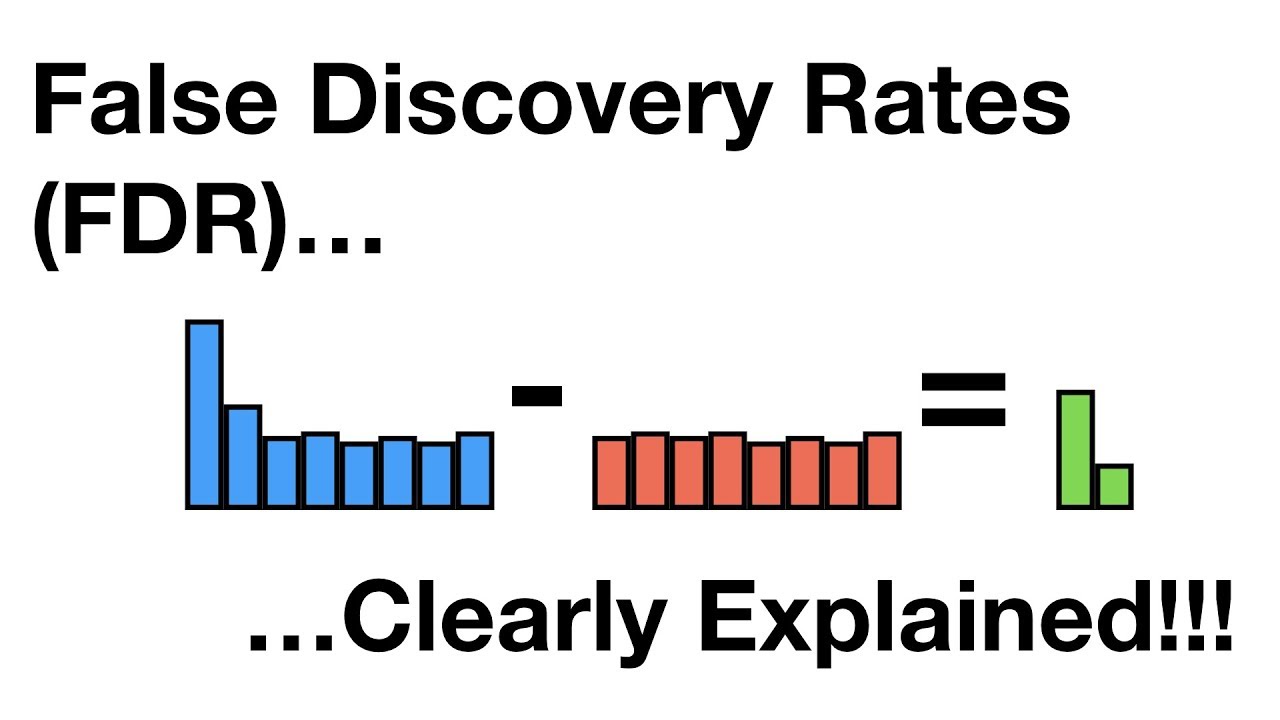
False Discovery Rates, FDR, clearly explained
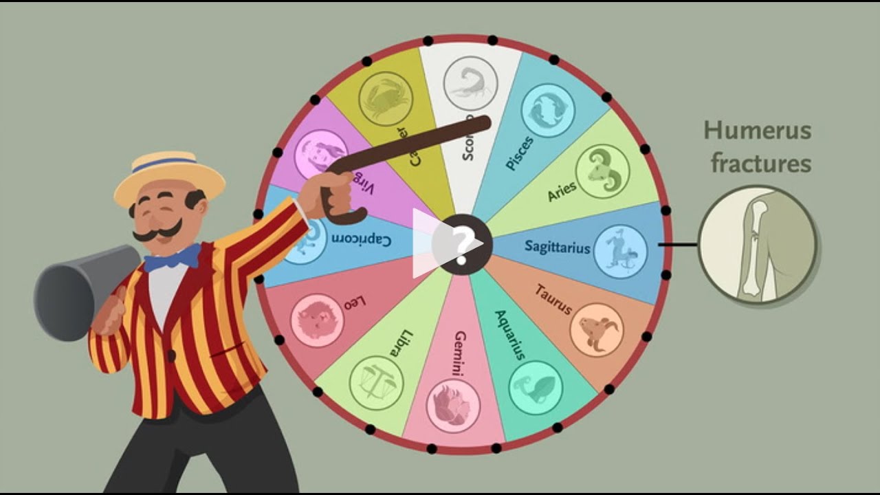
The Problem of Multiple Comparisons | NEJM Evidence
Type I error vs Type II error

ANOVA Part IV: Bonferroni Correction | Statistics Tutorial #28 | MarinStatsLectures
Errors and Power in Hypothesis Testing | Statistics Tutorial #16 | MarinStatsLectures
5.0 / 5 (0 votes)
Thanks for rating: