High School Physics: Kinematic Equations

Dan Fullerton

19 Aug 201110:55

EducationalLearning

32 Likes 10 Comments

TLDRThe video script introduces kinematic equations as essential tools for solving physics problems involving straight-line motion with constant acceleration. It focuses on five key variables: initial velocity (V₀), final velocity (V), displacement (ΔX), acceleration (a), and time (T). The script presents three primary kinematic equations and outlines a systematic problem-solving approach, emphasizing the importance of proper setup to efficiently solve motion problems. Through examples, including a racecar acceleration and a hammer drop on the moon, the video demonstrates how to apply these equations and highlights the ease of solving problems once the setup is complete.

Takeaways

📚 The discussion focuses on kinematic equations in physics for solving problems related to objects moving in a straight line at constant acceleration.
🛠️ Kinematic equations are efficient tools for solving motion problems, sometimes more so than graphs.
🎯 The five key variables in kinematic equations are initial velocity (V₀), final velocity (V), displacement (ΔX), acceleration (a), and elapsed time (T).
✍️ The three primary kinematic equations relate final velocity, displacement, and the square of final velocity to initial velocity, acceleration, and time.
📈 To effectively use kinematic equations, follow a specific problem-solving procedure: label the motion (horizontal or vertical), choose a positive direction, create a motion analysis table, and solve for the unknowns.
🚗 An example problem involves a racecar accelerating from rest at 4.9 m/s² and calculating its speed after traveling 200 meters.
🌙 A vertical motion example involves an astronaut on the moon dropping a hammer, calculating its acceleration after it falls 6 meters in 2.7 seconds.
🚀 The problem-solving process is straightforward but requires careful setup to avoid mistakes.
📊 Even without direct information on acceleration, one can solve for it and subsequently other variables using the appropriate kinematic equations.
🎢 The script encourages creating custom kinematics problems involving horizontal and vertical motion to practice problem-solving skills.

Q & A

What are the main topics discussed in the video?
-The main topics discussed in the video are kinematic equations in physics, specifically for objects moving in a straight line at a constant acceleration, and how to solve problems using these equations efficiently.
What are the five key variables in kinematic equations?
-The five key variables in kinematic equations are initial velocity (V naught), final velocity (V), displacement (Delta X or Delta Y for vertical motion), acceleration (a), and elapsed time (T).
How many kinematic equations are there, and what do they relate?
-There are three kinematic equations. The first relates final velocity to initial velocity, acceleration, and time. The second equates displacement to initial velocity times time plus half of acceleration times the square of time. The third equation links the square of final velocity to the square of initial velocity, plus two times acceleration times displacement.
What is the first step in solving motion problems using kinematic equations?
-The first step is to label the analysis for either horizontal or vertical motion, choosing a direction to be positive, and ensuring that the problem setup is consistent with this choice.
How does one choose a direction to be positive in kinematic problems?
-A direction is chosen to be positive based on the object's initial motion. It's best to be consistent in this choice to reduce the chance of error.
What is a motion analysis table, and how is it used in solving problems?
-A motion analysis table is a tool used to organize the known variables (V naught, V, Delta X/Y, a, and T) in a given problem. It helps in identifying which three variables are known and which two need to be solved for.
In the racecar example, what is the car's final speed after traveling 200 meters with an acceleration of 4.9 m/s^2?
-The car's final speed is 44.3 meters per second, considering the positive direction to the right.
How is the acceleration of the hammer dropped on the moon calculated in the example?
-The acceleration is calculated using the formula Delta Y equals 1/2 a t-squared, where Delta Y is 6 meters, and T is 2.7 seconds. The calculated acceleration is 1.6 meters per second squared.
In the second car problem, how is the distance traveled calculated when given initial velocity, final velocity, and time?
-The distance traveled is calculated using the formula Delta X equals V naught T plus 1/2 a t-squared. By first finding the acceleration (a = (V - V naught) / T) and then substituting the known values into the formula, the calculated distance is 216 meters.
What is the purpose of creating your own kinematic problem as suggested in the video?
-Creating your own kinematic problem helps to practice and reinforce the understanding of the kinematic equations and the problem-solving process. It encourages creative thinking and practical application of the concepts learned.
What additional advice does the speaker give for solving kinematic problems efficiently?
-The speaker advises to take the time to set up the problem properly, as this is key to solving it efficiently. It's important to label the analysis correctly, choose a consistent direction for positive values, and fill in the motion analysis table accurately to minimize errors.

Outlines

00:00

📚 Introduction to Kinematic Equations

This paragraph introduces the concept of kinematic equations in physics, focusing on their application to problems involving objects moving in a straight line at constant acceleration. It emphasizes the efficiency of these equations over graphical methods for certain problems and outlines the five key variables (initial velocity (V₀), final velocity (V), displacement (Δx), acceleration (a), and time (T)) that are central to these equations. The paragraph also previews the problem-solving process, highlighting the importance of proper setup in efficiently solving motion problems.

05:04

🚗 Solving Kinematic Problems - Horizontal Motion

This section delves into the specifics of solving horizontal kinematic problems using the previously mentioned variables and equations. It presents a step-by-step approach, starting with labeling the direction of motion, choosing a positive direction, and filling out a motion analysis table with known quantities. The paragraph demonstrates how to apply the kinematic equations to two sample problems: one involving a racecar accelerating from rest and another concerning an astronaut dropping a hammer on the moon. The detailed calculations and problem-solving techniques are provided, showcasing the practical application of the equations.

10:05

🤖 Creating and Solving Custom Kinematic Problems

The final paragraph encourages the learner to create their own kinematic problems, focusing on both horizontal and vertical motion scenarios. It provides a creative exercise where the learner is asked to design a problem with three given variables and solve for the remaining two. The paragraph suggests incorporating a story or interesting elements to enhance the learning experience and offers the resource of physics.com for additional help. This exercise aims to solidify the understanding of kinematic equations and problem-solving strategies.

Mindmap

Keywords

💡Kinematic Equations

Kinematic Equations are mathematical formulas used to predict the behavior of objects moving at constant acceleration along a straight line. In the context of the video, these equations are essential tools for solving physics problems involving motion. The video explains how to use these equations to determine variables such as initial velocity, final velocity, displacement, acceleration, and time elapsed, given a set of known values.

💡Constant Acceleration

Constant acceleration refers to the rate of change of velocity that remains the same over time. In the video, the concept is crucial for understanding how objects move in a straight line without any change in the acceleration. It is a key assumption that allows the use of kinematic equations to predict and analyze motion.

💡Displacement

Displacement is the change in position of an object and is a vector quantity that considers the direction of movement. In the context of the video, displacement is one of the five key variables used in kinematic equations to describe the straight-line motion of an object, whether horizontal or vertical.

💡Initial Velocity (V naught)

Initial velocity, often denoted as V naught, is the speed of an object at the beginning of its motion. It is a critical variable in kinematic equations, allowing us to calculate other motion-related variables such as final velocity and displacement. The video emphasizes the importance of initial velocity in solving problems related to motion.

💡Final Velocity (V)

Final velocity is the speed of an object at the end of a specified time interval or after it has undergone a certain displacement. It is a fundamental concept in kinematics and is used in conjunction with initial velocity, acceleration, and time to analyze motion. The video demonstrates how to calculate final velocity using the kinematic equations.

💡Acceleration (a)

Acceleration is the rate at which an object's velocity changes over time. It is a key concept in physics and is central to the kinematic equations. The video explains how to determine acceleration and uses it to solve for other variables in motion problems, such as displacement and final velocity.

💡Elapsed Time (T)

Elapsed time refers to the total time that has passed during an object's motion. In the context of the video, time is one of the five key variables used in kinematic equations to analyze motion. Understanding the time elapsed is crucial for calculating other motion variables, such as displacement and final velocity.

💡Motion Analysis

Motion analysis is the process of studying and analyzing the motion of an object to determine its various motion-related variables. In the video, motion analysis involves creating a table with the known values and using kinematic equations to solve for the unknowns. It is a systematic approach to solving physics problems involving motion.

💡Problem Solving Steps

Problem Solving Steps refer to the structured procedure or sequence of actions taken to solve a problem. In the video, these steps are crucial for efficiently solving kinematics problems by setting up the problem correctly and systematically applying the kinematic equations to find the unknown variables.

💡Horizontal and Vertical Motion

Horizontal and vertical motion refer to the direction of an object's movement. Horizontal motion is along a straight line parallel to the ground, while vertical motion is along a straight line perpendicular to the ground. The video emphasizes the importance of distinguishing between these two types of motion when solving kinematics problems and using the appropriate kinematic equations.

Highlights

Introduction to kinematic equations in physics for solving problems related to objects moving in a straight line at constant acceleration.

Discussion on the efficiency of using graphs versus kinematic equations for solving motion problems.

Explanation of five key variables in kinematics: initial velocity (V naught), final velocity (V), displacement (Delta X or Delta Y), acceleration (a), and elapsed time (T).

Presentation of three fundamental kinematic equations and their applications.

Emphasis on the importance of proper setup in solving kinematic problems efficiently.

Procedure for solving motion problems, including labeling analysis, choosing a positive direction, and creating a motion analysis table.

Sample problem of a racecar accelerating from rest and calculating its speed after a given displacement.

Explanation of how to use the kinematic equations with a real-world example of a racecar's acceleration and displacement.

Illustration of solving for an unknown variable in kinematics by choosing the appropriate equation based on known quantities.

Second sample problem involving an astronaut on the moon and calculating the acceleration of a falling hammer.

Application of kinematic equations to a vertical motion problem to find the acceleration of an object.

Third sample problem about a car accelerating on a straight road and finding the distance traveled given initial and final velocities and time.

Demonstration of solving for acceleration and then displacement using the kinematic equations for a horizontal motion problem.

Encouragement for learners to create their own horizontal and vertical kinematics problems, providing practice and creative problem-solving opportunities.

Advice for learners to check aplusphysics.com for more help if needed.

Concluding remarks highlighting the importance of setup in solving kinematic problems and encouraging practice.

Transcripts

Browse More Related Video

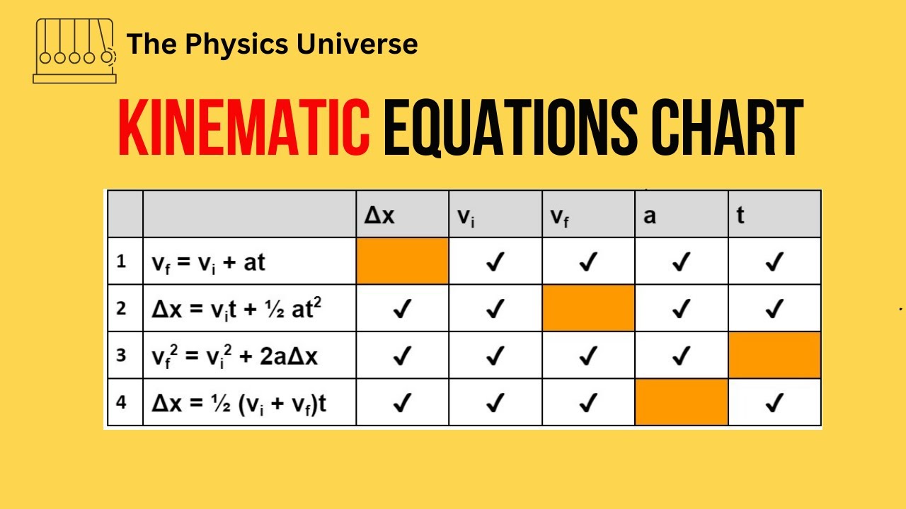
Creating And Using Kinematic Equations Chart - Kinematics - Physics

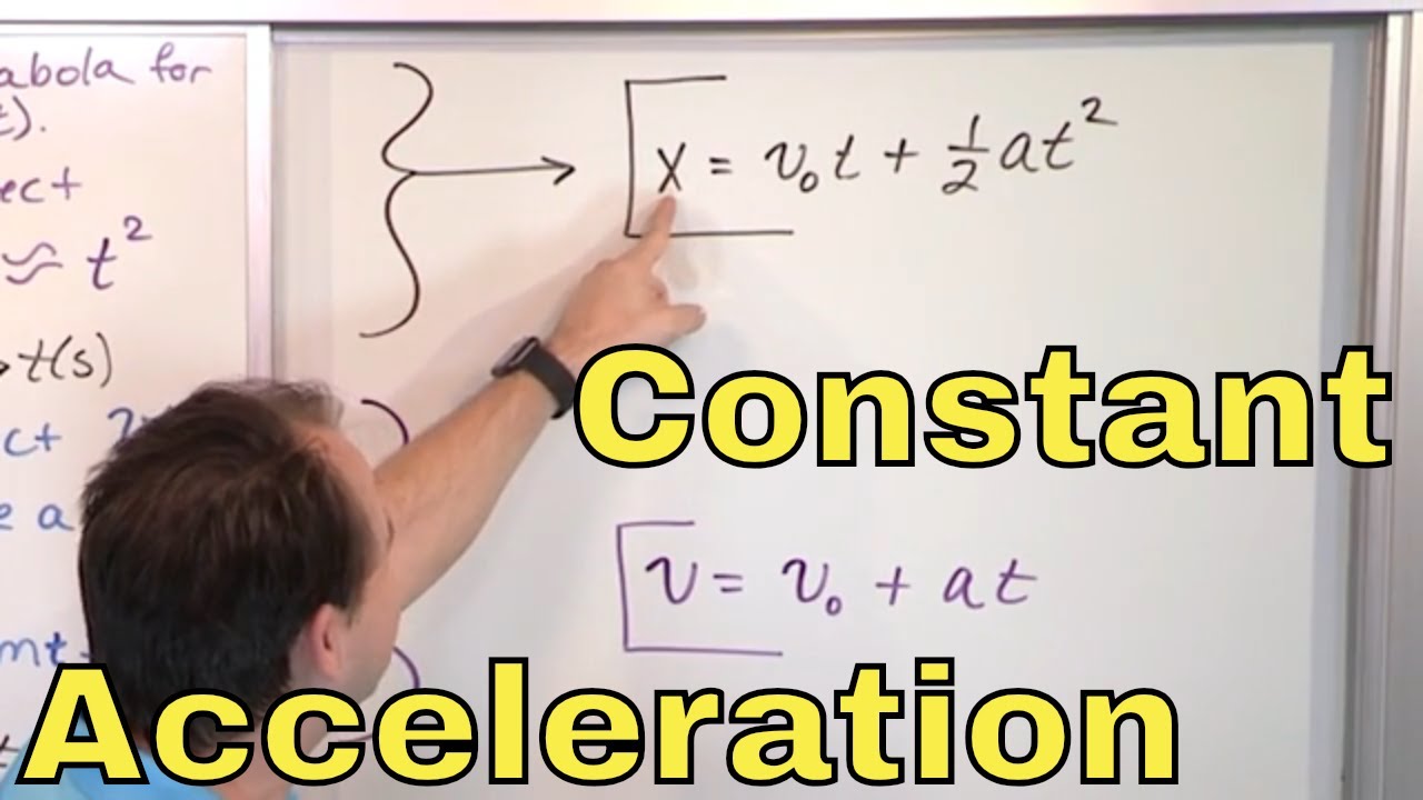
01 - Motion with Constant Acceleration in Physics (Constant Acceleration Equations)

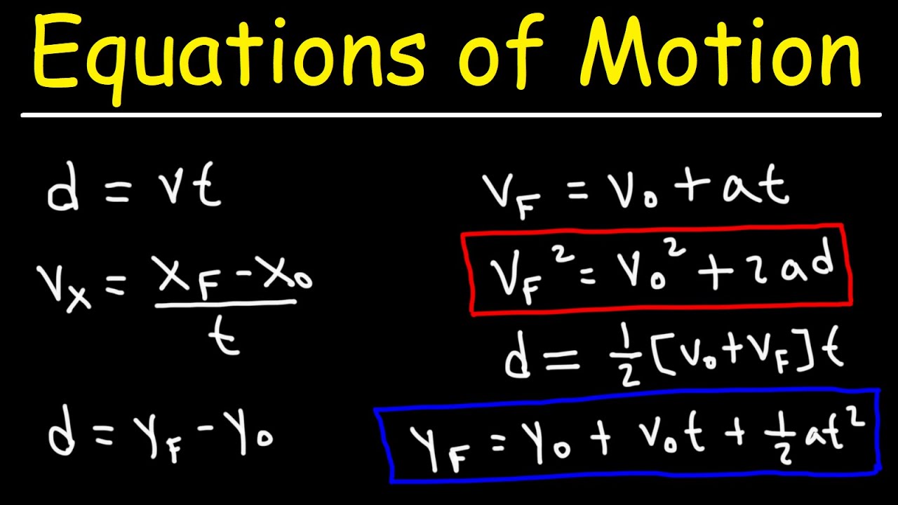
Equations of Motion

Equations of Motion by Graphical Method

College Physics 1: Lecture 10 - Solving 1-D Motion Problems

Rotational kinematic formulas | Moments, torque, and angular momentum | Physics | Khan Academy

High School Physics: Kinematic Equations

Takeaways

Q & A

What are the main topics discussed in the video?

What are the five key variables in kinematic equations?

How many kinematic equations are there, and what do they relate?

What is the first step in solving motion problems using kinematic equations?

How does one choose a direction to be positive in kinematic problems?

What is a motion analysis table, and how is it used in solving problems?

In the racecar example, what is the car's final speed after traveling 200 meters with an acceleration of 4.9 m/s^2?

How is the acceleration of the hammer dropped on the moon calculated in the example?

In the second car problem, how is the distance traveled calculated when given initial velocity, final velocity, and time?

What is the purpose of creating your own kinematic problem as suggested in the video?

What additional advice does the speaker give for solving kinematic problems efficiently?