Area Between Two Curves

The Organic Chemistry Tutor

19 Apr 202148:58

EducationalLearning

32 Likes 10 Comments

TLDRThis educational video tutorial provides a comprehensive guide on calculating the area between two curves using calculus. It begins by explaining the basics of finding the area under a single curve through definite integration. The tutorial then advances to discussing how to calculate the area between two curves by integrating the difference of the two functions over a specific interval. The explanation covers both functions in terms of x and y, providing viewers with a versatile understanding of the concept. Additionally, the video includes practice problems with step-by-step solutions, ranging from simple integrations to more complex scenarios involving linear and quadratic functions, ensuring viewers can apply these principles to solve real-world problems effectively.

Takeaways

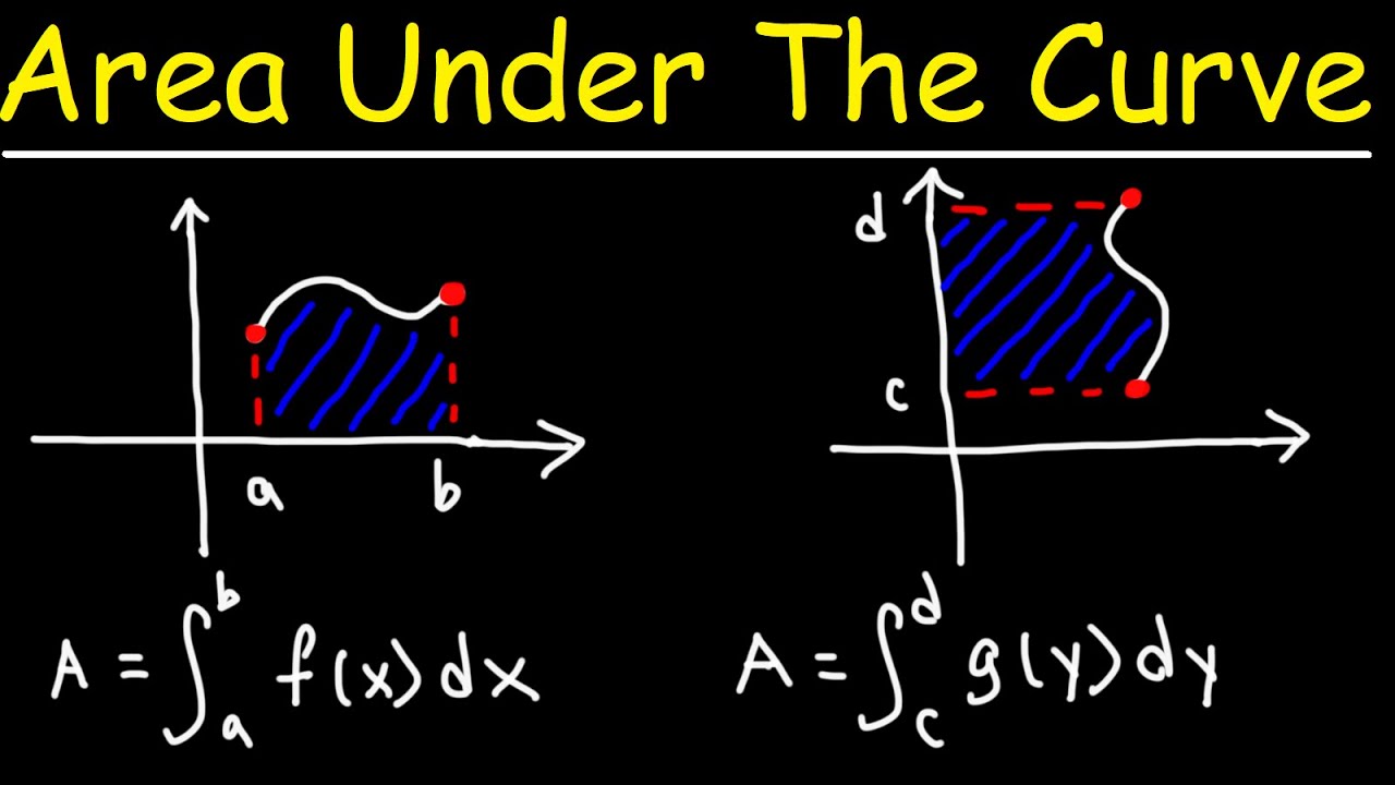
💡 The area under a curve from points a to b can be found by taking the definite integral of the function f(x) from a to b.
📖 To calculate the area between two curves, subtract the area under the lower curve from the area under the upper curve, essentially integrating the difference f(x) - g(x) from a to b.
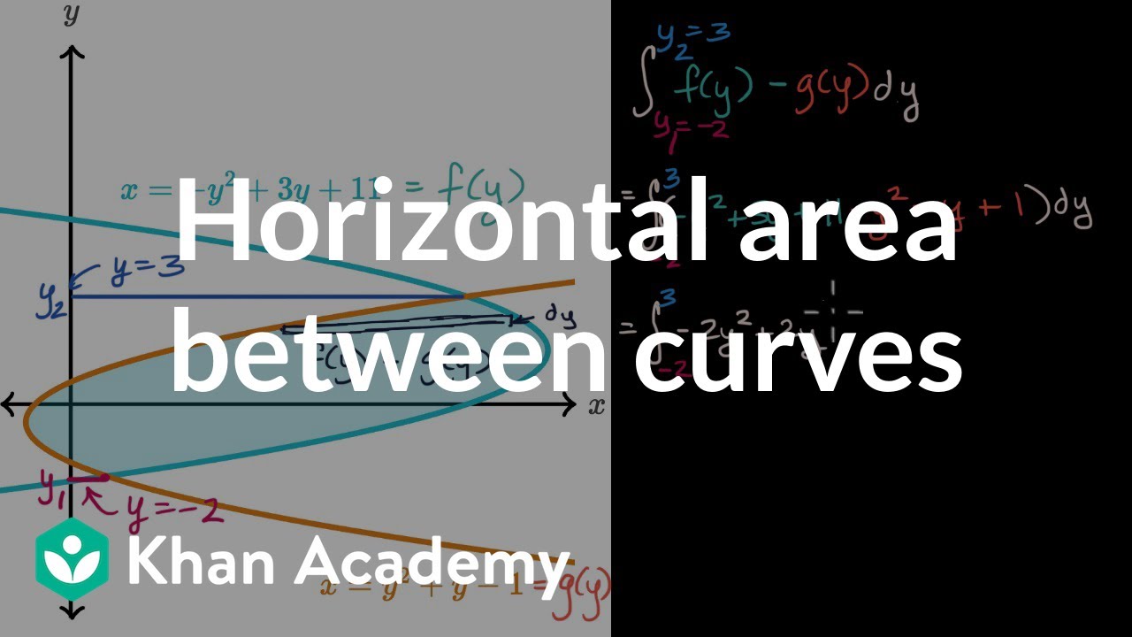
🔬 When dealing with functions of y (f(y)), the concept remains the same: integrate the difference between two functions from c to d to find the area between them.
📈 The area calculation can be applied in both the x and y directions, requiring adjustment of the functions to either y = f(x) or x = f(y) depending on the orientation.
🚡 For linear equations, geometric solutions (like using the formula for the area of a triangle) can sometimes offer a quicker path to finding areas, though calculus provides a universal approach.
📉 In practice, the process often involves finding points of intersection between curves to set the limits of integration for calculating the area between those curves.
📚 Factoring and solving quadratic equations can be necessary steps in determining the limits of integration when curves intersect.
📗 Calculating areas in terms of x versus y might require transforming equations, but the final area result remains consistent regardless of the approach.
📌 Intersection points between curves are critical in setting up the definite integral for area calculation, as these points often serve as the limits of integration.
💧 Integration techniques and understanding of antiderivatives play a key role in solving for areas under or between curves in calculus.

Q & A

How do you calculate the area between two curves?
-To calculate the area between two curves, you need to take the integral from a to b of the difference between the two functions (f(x) - g(x)) dx. The top function (f(x)) is subtracted by the bottom function (g(x)) over the interval [a, b].
Can the method of finding the area between two curves be applied to functions of y?
-Yes, the method can be applied to functions of y. When dealing with functions in terms of y (f(y) and g(y)), you integrate from c to d of the right function minus the left function (f(y) - g(y)) dy, to find the area between the curves.
How can you find the area of a region bounded by a curve and the x-axis?
-To find the area of a region bounded by a curve and the x-axis, calculate the definite integral of the function (f(x)) from the lower bound (a) to the upper bound (b). This gives the area under the curve between points a and b.
What is the significance of determining the top and bottom functions when finding the area between two curves?
-Determining the top and bottom functions is crucial because the area between two curves is found by integrating the difference between these functions. Subtracting the bottom function from the top ensures accurate calculation of the bounded area.
How do you determine the points of intersection when calculating the area between two curves?
-To determine the points of intersection between two curves, set the equations of the curves equal to each other and solve for x (or y, depending on the variable). These solutions give the bounds for integration and are essential for calculating the exact area between the curves.
In the context of integrating functions of y to find area, what does it mean to integrate the function on the right minus the function on the left?
-When integrating functions of y, 'integrating the function on the right minus the function on the left' means calculating the integral of the difference between the rightmost function (f(y)) and the leftmost function (g(y)) across an interval [c, d]. This method is used when the area of interest lies between curves described by functions of y, not x.
What steps are involved in converting an equation from x = f(y) to a function of y when calculating area?
-To convert an equation from x = f(y) to a function of y, you rearrange the equation to solve for y, making y the subject. This might involve algebraic manipulations such as adding, subtracting, multiplying, dividing, or factoring. The result is an expression where y is expressed in terms of x, which can then be used for integration.
How do you use geometry to find the area of a region bounded by lines and curves?
-Geometry can be used to find the area of simple geometric shapes (like triangles or rectangles) bounded by lines and curves by applying formulas, such as 1/2 base times height for triangles. For more complex shapes bounded by curves, calculus methods involving definite integrals are typically used.
Why might the method for calculating area differ when dealing with functions of x versus functions of y?
-The method for calculating area differs between functions of x and functions of y due to the orientation of the curves with respect to the coordinate axes. For functions of x, the curves extend vertically and the area is calculated along the x-axis. For functions of y, the curves extend horizontally, and the area is calculated along the y-axis. This difference affects how the integration bounds and differences between functions are determined.
What is the process for finding the area of a region bounded by a curve and the y-axis?
-To find the area of a region bounded by a curve and the y-axis, you calculate the definite integral of the curve's equation from the lower bound (c) to the upper bound (d) in terms of y. This integral gives the area to the left or right of the y-axis, depending on the curve's orientation and the limits of integration.

Outlines

00:00

📘 Introduction to Calculating Areas Between Curves

This segment introduces the fundamental concept of calculating the area between curves, focusing on the difference between areas under two functions defined from a to b. The approach starts with calculating the area under a single curve as the definite integral of the function over a specified interval. It then extends to finding the area between two curves by taking the definite integral of the difference between the two functions over the interval. The explanation is made concrete with an example involving functions f(x) and g(x), highlighting the procedure for both cases where the functions are defined in terms of x and when defined in terms of y, illustrating the versatility of the method.

05:02

📐 Practical Example: Linear Function and Axis Intersection

This part provides a practical example involving the calculation of the area bounded by a linear function, y-axis, and x-axis, illustrating both geometric and calculus-based methods for area calculation. By depicting a triangle formed by the line y = 8 - 2x and the axes, it initially calculates the area using the formula for the area of a triangle. Subsequently, it delves into the calculus approach by integrating the function from 0 to 4, demonstrating the consistency of results between the two methods. The example underscores the applicability of calculus in determining areas in graphical contexts.

10:03

📉 Calculating Area Between a Line and a Parabola

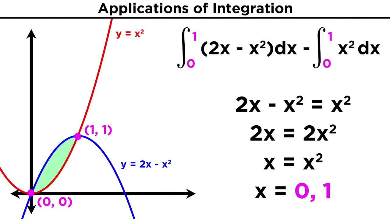
This section tackles a more complex scenario involving the calculation of the area between a line, y = x, and a parabola, y = x^2, emphasizing the determination of the intersection points as a preliminary step. Through setting the equations equal to each other and factoring, the intersection points are found, enabling the calculation of the area between the curves by integrating the difference between the functions over the identified interval. This example highlights the process of identifying the 'top' and 'bottom' functions to accurately compute the area between them.

15:08

🔍 Exploring Areas with Quadratic and Radical Functions

This segment explores calculating areas involving quadratic and radical functions, y = x^2 and x = y^2, illustrating how to graph these functions and identify the bounds of the area to be calculated. The narrative guides through the process of setting equal the functions in terms of x and y, solving for the intersection points, and then integrating the difference between the functions over the interval defined by these points. The explanation is detailed, covering the steps to transform functions and solve for areas in different function forms.

20:11

📊 Area Calculation Between Two Parabolas

Focusing on the calculation of the area between two parabolas defined in terms of y, this part sets the stage by graphing x = y^2 - 1 and x = 1 - y^2 to find their intersection points. The narrative proceeds with setting the equations equal, solving for y, and then integrating the difference between the two functions across the interval determined by the intersection points. This example provides insights into handling cases where functions are defined in terms of y, illustrating the steps to graph, solve, and calculate areas in such contexts.

25:13

📚 Advanced Practice with Parabolic and Linear Equations

In this more advanced example, the focus shifts to calculating the area of a region bounded by a parabolic curve, y = x^2 - 4x, and the x-axis. The segment elaborates on finding the x-intercepts and the vertex of the parabola to graph it accurately. It then discusses calculating the area using calculus by identifying the top (x-axis) and bottom (curve) functions and integrating the difference between them from 0 to 4. This advanced practice demonstrates integrating more complex functions and the importance of graphical representation in understanding the bounded area.

30:15

📝 Complex Area Calculation Between Linear and Parabolic Curves

This piece presents a complex scenario involving the calculation of the area between a parabolic curve, y = x^2 - 4x, and a linear function, y = 6 - 3x. The section meticulously details finding the points of intersection between the curves and then proceeds to calculate the area bounded by these functions. Through integrating the difference between the linear (top function) and parabolic (bottom function) equations over the determined interval, this example showcases the intricate process of calculating areas in scenarios involving both linear and nonlinear functions.

35:18

🎓 Area Between Parabola and Linear Function in Different Quadrants

The final section introduces a scenario calculating the area between a parabola opening to the right and a linear function, using the equations x = y^2 - 4 and x = 3y - 2. The explanation involves graphing these functions, finding their points of intersection by setting the equations equal, and factoring to solve. The process culminates in integrating the difference between the functions over the identified interval. This concluding example reinforces the diversity of graphical scenarios for area calculation, emphasizing problem-solving in varying function contexts.

Mindmap

Keywords

💡Definite Integral

The definite integral is a fundamental concept in calculus that represents the accumulation of quantities, often visualized as the area under a curve on a graph. In the video, it is primarily used to calculate the area under a single curve or between two curves by integrating a function or the difference of two functions across a specific interval. The process involves finding the antiderivative of the function(s) and evaluating it at the upper and lower bounds of the interval. For example, the area under a curve from a point 'a' to 'b' is found by calculating the definite integral of the function representing the curve from 'a' to 'b'.

💡Area between Curves

This term refers to the region enclosed between two curves on a graph. The video explains that to find this area, one must integrate the difference between the upper function (f(x)) and the lower function (g(x)) over the interval from 'a' to 'b'. This method allows for the calculation of the net area enclosed between the curves, accounting for the orientation of each curve relative to the x-axis. Examples provided in the video include calculating the area between linear and quadratic functions, illustrating how this concept applies to both simple and complex regions.

💡Top Function and Bottom Function

In the context of calculating the area between two curves, the 'top function' is the one that lies above the 'bottom function' over the interval of integration. The distinction is crucial for setting up the integral correctly, as the video illustrates by subtracting the bottom function from the top function. This setup ensures that the calculated area is always positive, as it accounts for the relative positions of the functions on the graph. Examples of identifying and using top and bottom functions were shown through various practice problems in the video.

💡Antiderivative

An antiderivative of a function is another function whose derivative is the original function. It plays a central role in finding definite integrals, as shown in the video, because calculating the area under a curve or between curves involves finding the antiderivative of the function(s) involved. The video demonstrates how to find the antiderivative of simple functions like polynomials and then use these antiderivatives to evaluate the integral at the bounds, which directly contributes to finding areas.

💡Integration by Geometry

The video highlights that in some cases, especially when dealing with linear functions forming simple geometric shapes like triangles, the area can be calculated directly using geometric formulas. This approach provides a quick and intuitive method for finding areas without the need for integral calculus, serving as a validation for more complex integral calculations. An example given in the video involves calculating the area of a triangle formed by a linear equation and the coordinate axes.

💡Function of y

The concept of expressing a function in terms of y, rather than the more conventional x, is discussed in the video as an alternative approach to calculating areas. This method is useful when the region of interest is better described or bounded by vertical lines, making it easier to integrate with respect to y. The video shows how to convert a function of x into a function of y for this purpose and then how to integrate this function over a given interval along the y-axis.

💡Points of Intersection

Points of intersection are the coordinates at which two curves cross each other on a graph. These points are critical for defining the limits of integration when calculating the area between the curves, as they mark the start and end points of the region of interest. The video demonstrates how to find these points algebraically by setting the equations of the curves equal to each other and solving for x or y, and then uses these points as the bounds for the definite integrals.

💡X-axis and Y-axis Intercepts

Intercepts are the points where a curve crosses the x-axis or y-axis. In the context of the video, intercepts are used to understand the geometry of the curves and to set up the bounds for integration. Specifically, x-axis intercepts help in determining the limits for integration when calculating the area under a curve or between curves. The video illustrates finding these intercepts for linear and quadratic functions as part of the process of sketching the curves and setting up the area calculations.

💡Zero Product Property

This mathematical principle is used in the video to find the points of intersection between curves. It states that if a product of two expressions is zero, then at least one of the expressions must be zero. The video applies this property to factor and solve polynomial equations resulting from setting two curve equations equal to each other, which in turn helps in determining the limits of integration for calculating areas.

💡Power Rule for Integration

The power rule is a basic technique for finding the antiderivative of a power function. It states that the antiderivative of x^n is (x^(n+1))/(n+1), provided that n is not equal to -1. This rule is frequently employed in the video's examples, where it's used to calculate the antiderivatives of polynomial functions as a step in finding the area under curves or between curves. This demonstrates the rule's utility in simplifying the integration process for functions expressed in terms of power of x (or y).

Highlights

Introduction to calculating the area between two curves, emphasizing the difference between integrating over x and y axes.

Explaining the basic concept of finding the area under a single curve using definite integrals.

Introducing the method for calculating the area between two curves by taking the integral of the difference of their functions.

Differentiating between functions of x and functions of y for calculating areas and demonstrating the respective approaches.

Practice problem: Calculating the area of a region bounded by a linear equation, the x-axis, and the y-axis, using both geometric and calculus methods for verification.

Demonstration of solving for x in terms of y to calculate areas related to the y-axis, introducing a reverse method for integrating with respect to y.

Solving a problem that involves finding the area between a line and a parabola, showcasing the process of determining points of intersection and integrating between these points.

Tackling a more complex area calculation between two curves that intersect at more than one point, applying the method of subtracting the lower function from the upper function.

Applying the concept to find the area bounded by curves in the first quadrant, emphasizing the role of intersection points in setting integration limits.

Addressing a scenario with horizontally shifted parabolas to calculate the area between them, highlighting the importance of understanding curve transformations.

Illustrating the calculation of area under a shifted parabola relative to the x-axis, showcasing how to apply integration techniques to polynomial functions.

Exploring the area between a parabola and a linear function, stressing the need for identifying intersection points and correctly determining the upper and lower functions.

Describing the process of calculating the area between two curves represented by different equations, including a parabolic and a linear equation.

Demonstrating the approach for integrating functions of y to find areas between curves that open sideways, using points of intersection as integration limits.

Final example emphasizing the complexity of determining areas between curves with multiple intersection points, including the use of factoring and setting up the correct integral bounds.

Transcripts

Browse More Related Video

Finding the Area Between Two Curves by Integration

Finding The Area Under The Curve Using Definite Integrals - Calculus

Calculus 1: Area Between Curves Examples

Calculus AB Homework 7.3 Area Between Curves

Area Between Two Curves

Horizontal area between curves | Applications of definite integrals | AP Calculus AB | Khan Academy

Related Tags

Mathematics Calculus Area Calculation Function Analysis Definite Integral Practice Problems Educational Study Guide Graphing Techniques Tutorial