What do quadratic approximations look like
TLDRThis video script delves into the concept of local linearization and introduces quadratic approximations. It explains how a flat plane can be used to approximate a function near a specific point, and then advances to discuss how a more complex surface, resembling a parabola when sliced, can provide a closer approximation. The script promises a deeper exploration of how to adjust constants to achieve a tight fit to the original function's graph, emphasizing the improved accuracy of quadratic over linear approximations.
Takeaways
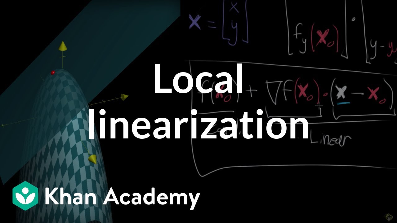
- 📈 The script discusses the concept of local linearization of a function and its graphical interpretation as a tangent plane to the graph at a specific point.
- 📚 The speaker introduces the idea of quadratic approximations as an extension of local linearization, offering a more precise fit to the function's graph near a chosen point.
- 📊 Quadratic approximations are represented graphically as surfaces that closely follow the original function's graph, appearing as parabolas when sliced in various directions.
- 🔍 The script explains that the shape of the quadratic approximation can vary depending on the direction of the slice, showing concave up or concave down parabolas.
- 📐 The approximation's accuracy is highlighted as being very close to the actual function near the point of approximation but deviating as one moves further away.
- 🔢 The script differentiates between linear functions, which are planes, and quadratic functions, which include terms with variables squared or multiplied together.
- 📉 Linear functions are described as having a constant and linear terms involving variables x and y, with an additional constant term making it affine rather than strictly linear.
- 📈 Quadratic functions include the same linear terms as linear functions but also add quadratic terms, which are products of two variables or squared variables.
- 🔑 The script emphasizes the increased control over the fit of the approximation by adjusting the constants in the quadratic function, which depends on the specific point of approximation.
- 🔍 The importance of partial derivatives in determining the optimal constants for the quadratic approximation is mentioned, hinting at a process similar to local linearization but with added complexity.
- 🔄 The speaker promises to cover in the next videos how to tweak the constants to achieve a close fit to the curve, indicating a continuation of the topic.
Q & A
What is the local linearization of a function?
-Local linearization of a function is the process of approximating a function near a specific point using a linear function. Graphically, it can be visualized as a tangent plane to the function's graph at that point.
Why is local linearization useful?
-Local linearization is useful because it provides a simpler way to approximate a function near a specific point. This can make it easier to analyze and work with the function in that region.
What is a quadratic approximation?
-A quadratic approximation is a more accurate method of approximating a function near a specific point. It uses a quadratic function, which includes terms up to the second degree, to hug the graph of the original function more closely than a linear approximation.
How does a quadratic approximation differ from a local linearization?
-A quadratic approximation differs from a local linearization by including additional terms that account for curvature. While a local linearization uses a tangent plane, a quadratic approximation uses a surface that can bend to match the function's curvature more closely.
What does the graph of a quadratic approximation look like?
-The graph of a quadratic approximation looks like a surface that closely follows the original function's graph near the point of approximation. It can vary in appearance, looking like a concave up or concave down parabola depending on the direction of the slice.
What terms are included in a quadratic function?
-A quadratic function includes a constant term, linear terms (like x and y), and quadratic terms (like x^2, y^2, and xy). These terms allow for a more detailed approximation that can better match the original function's shape.
How does the inclusion of quadratic terms improve the approximation?
-The inclusion of quadratic terms improves the approximation by allowing the function to account for changes in curvature. This results in a more accurate representation of the original function near the point of approximation.
What are the benefits of using a quadratic approximation over a linear one?
-The benefits of using a quadratic approximation over a linear one include a closer fit to the original function and more accurate results over a wider range near the point of approximation. This is because the quadratic approximation can better capture the function's curvature.
What kind of information is needed to create a quadratic approximation?
-To create a quadratic approximation, you need information about the function's value, first derivatives, and second derivatives at the point of approximation. This includes partial differential information that describes how the function changes in multiple directions.
What will be discussed in the next videos following this one?
-The next videos will discuss how to adjust the six constants in a quadratic function to create an approximation that closely matches the original function's curve at different points. This involves understanding and applying partial differential information.
Outlines
📚 Introduction to Local Linearization and Quadratic Approximations
This paragraph introduces the concept of local linearization of a function, explaining it as a tangent plane to a graph at a specific point to approximate the function's behavior near that point. The narrator then transitions to the main topic of the video, which is quadratic approximations. These are a more advanced form of approximation that, unlike linear approximations, can provide a surface that closely follows the original function's graph, resembling a parabola when sliced in any direction. The paragraph sets the stage for a deeper dive into the graphical and formulaic aspects of quadratic approximations in subsequent videos.
Mindmap
Keywords
💡Local Linearization
💡Graph
💡Quadratic Approximations
💡Tangent Plane
💡Parameters
💡Surface
💡Parabolas
💡Multiple Dimensions
💡Affine Function
💡Quadratic Terms
💡Partial Differential
Highlights
Local linearization of a function is explained with a nice graphical interpretation.
A flat plane tangent to the original graph at a specific point is used for local linear approximation.
Quadratic approximations are introduced as the next level beyond linear approximations.
Graphical representation of quadratic approximations involves a surface that hugs the graph more closely.
Quadratic approximations can look different when viewed from different angles, appearing concave up or down.
Quadratic approximations carry more information and provide a closer fit to the graph than linear approximations.
A linear function is represented by a plane with a constant term and linear terms in x and y.
Quadratic terms include x squared, y squared, and xy, allowing for more control in fitting the curve.
Tweaking the constants in a quadratic function enables it to closely hug the curve at a specific point.
The optimal plane or surface for approximation depends on the specific point chosen on the graph.
Partial differential information about the original function is crucial for determining the best fit.
Upcoming videos will discuss how to adjust the six constants in a quadratic function for optimal approximation.
Quadratic approximations provide a more accurate representation of the function near the point of interest.
The approximation deviates from the graph only when moving far away from the original point.
Quadratic approximations, despite being more complex, offer a closer fit to the original function.
The video series will delve deeper into the process of quadratic approximation and its practical applications.
Transcripts
Browse More Related Video

5.0 / 5 (0 votes)
Thanks for rating: