Tensor Calculus 6: Differential Forms are Covectors
TLDRThis video explores the concept of differential forms as covector fields, building on the understanding of covectors as entities that take vectors to scalars. It reinterprets differentials not just as small changes, but as operators that transform scalar fields into covector fields, represented by level sets. The video explains how these covector fields act on vectors, obey linearity laws, and geometrically represent the directional derivative of a function, providing a deeper insight into the relationship between differentials and integrals.
Takeaways
- 📚 Differential forms are re-introduced as covector fields, building upon the concept of 'Covectors' from an earlier video in the 'Tensors for Beginners' series.
- 🔍 The 'd' symbol in differentials is reinterpreted from signifying a small change to being an operator that turns a scalar field into a covector field.
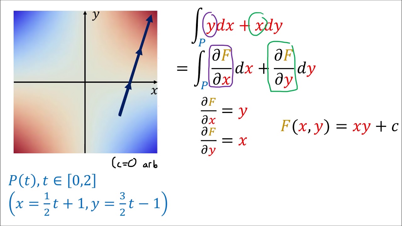
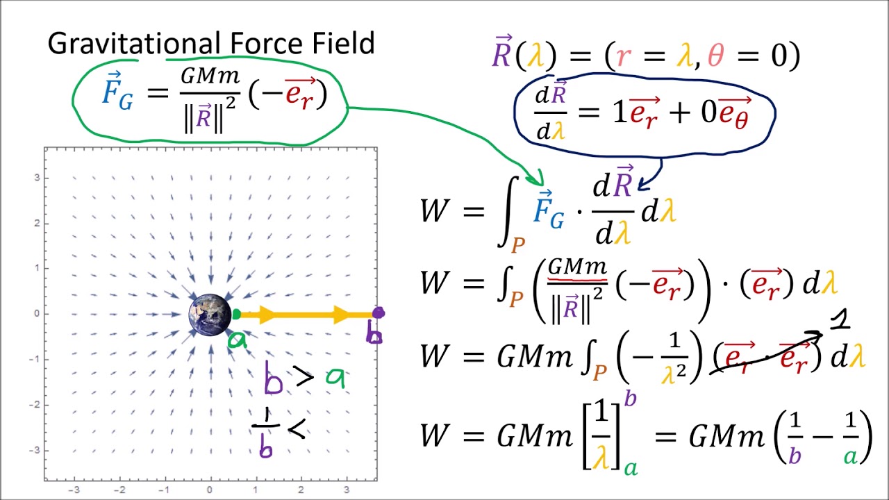
- 📉 Differentials are explained through the calculation of area under a curve, using infinitesimally small rectangles and the limit process to define the integral.
- 📚 Covectors are described as oriented stacks that take vectors as input and produce scalars as output by counting the number of lines pierced by the vector.
- 📐 The linearity properties of covectors are highlighted, emphasizing the ability to add inputs or outputs and scale inputs or outputs to achieve the same result.
- 🌐 The concept of scalar fields and covector fields is introduced, with scalar fields assigning a scalar to every point in space and covector fields assigning a covector to every point.
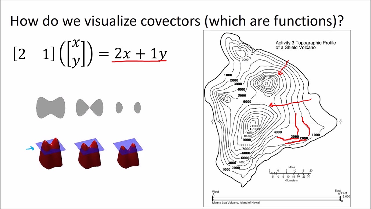
- 📈 The process of obtaining a covector field from a scalar field is illustrated through the tracing of level sets, which are curves of constant value.
- 📊 Examples of covector fields for dx, dy, dr, and dθ are given, showing how they represent level sets in different coordinate systems.
- 🔢 The action of a covector field df on a vector v is explained, demonstrating how to calculate the result by considering the covector at the point where the vector is located.
- 📏 The geometrical interpretation of df(v) is discussed, revealing it as the directional derivative of the function f with respect to the velocity vector v, indicating the rate of change of f in the direction of v.
- 🔄 The video concludes with the understanding that df(v) measures both the steepness of the function f and the length of the velocity vector v, providing insight into the rate of change of f at a point.
Q & A
What is the main topic of the video?
-The main topic of the video is the relationship between differential forms and covector fields, and how differentials can be reinterpreted as covectors.
What is the prerequisite knowledge for understanding this video?
-The prerequisite knowledge is understanding what a covector is, which can be found in the 'Tensors for Beginners' series video titled 'What are Covectors?'.
What are differentials in the context of integrals?
-In the context of integrals, differentials represent infinitesimally small changes in a variable, often seen on the right-hand side of integrals as 'dx'.
How are covectors described in the script?
-Covectors are described as stacks of lines that take a vector as input and produce a scalar as output by counting the number of lines pierced by the vector.
What is the reinterpretation of the 'd' symbol in differentials presented in the video?
-The 'd' symbol is reinterpreted as an operator that takes a scalar field and outputs a covector field, rather than just representing a small change in a variable.
How does a change of variables in an integral relate to differentials?
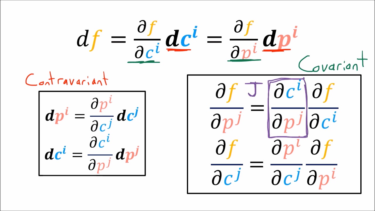
-A change of variables in an integral involves using the relationship between differentials, such as 'du/dx = cos(x)', to convert one differential into another based on the slope of the function in a small region.
What are the two linearity properties that covectors obey?
-The two linearity properties are: 1) adding the inputs or adding the outputs of a covector yields the same result, and 2) scaling the input or scaling the output of a covector yields the same result.
How are scalar fields and covector fields related in the video?
-Scalar fields are spaces where a scalar is assigned to every point, while covector fields are spaces where a covector is assigned to every point, and are obtained by tracing out the level sets of the scalar function.
What is the geometrical interpretation of df(v) in the context of the video?
-The geometrical interpretation of df(v) is the directional derivative of the function f with respect to the velocity vector v, indicating the rate of change of f at a point when moving with velocity v.
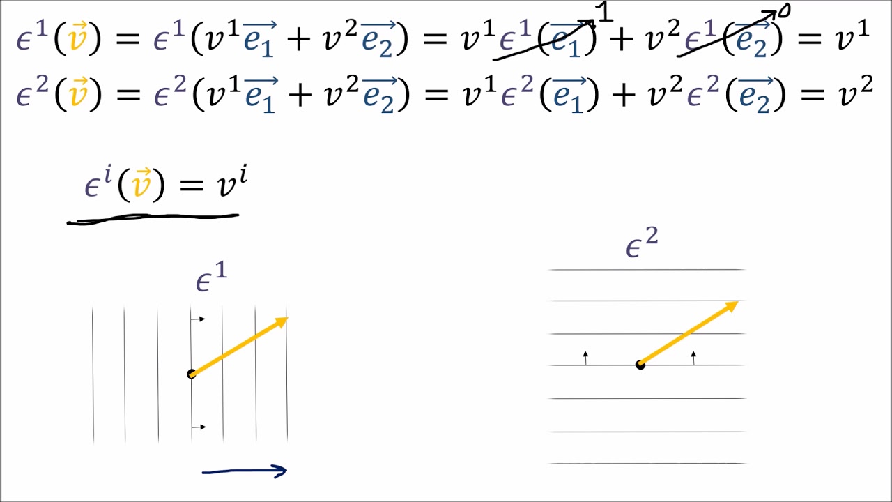
How does the video explain the calculation of df(v) for a given vector v?
-The video explains that to calculate df(v), one must look at the covector at the point where the vector v is located, and then count how many stack lines v pierces for that covector.
What is the significance of the level set curves in the context of covector fields?
-Level set curves are significant because they represent the curves of constant value in a scalar field, and the orientation of these curves gives the direction of the covector field.
Outlines
📚 Introduction to Differential Forms and Covectors
This paragraph introduces the concept of differential forms, explaining their relationship to covector fields. It suggests watching a previous video for a foundational understanding of covectors, which are described as structures that take a vector and produce a scalar. The paragraph sets the stage for a deeper exploration of differentials, hinting at a reinterpretation of the 'd' symbol and its role in connecting differentials and covectors. It also reviews the concept of differentials in the context of integrals and change of variables, using the example of the area under a curve and variable transformation in integration.
🔍 Reinterpreting Differentials as Covector Fields
The second paragraph delves into the reinterpretation of the 'd' symbol in differentials, suggesting that 'd' is not just a representation of a small change, but an operator that turns a scalar field into a covector field. It explains the concept of level sets in scalar fields and how they relate to covector fields, using visual examples to illustrate the orientation of these fields. The paragraph also introduces the terminology of '0-forms' for scalar fields and '1-forms' for covector fields, and discusses the algebraic representation of this transformation, including examples of dx, dy, dr, and dθ in different coordinate systems.
📐 Calculating Covector Field Outputs and Their Linearity
This paragraph explains how to calculate the output of a covector field acting on a vector, emphasizing the importance of considering the covector at the specific point where the vector is located. It illustrates this with examples, showing how the output is determined by counting the number of stack lines pierced by the vector. The paragraph also discusses the linearity properties of covector fields, demonstrating how inputs and outputs can be added or scaled to achieve the same result, and introduces the geometric interpretation of df(v) as the directional derivative of a function f in the direction of a vector v.
🌐 Geometric Interpretation and Future Exploration
The final paragraph wraps up the discussion by summarizing the geometric interpretation of df(v) as the directional derivative, highlighting how it measures the rate of change of a function at a point when moving with a certain velocity. It uses the analogy of a mountain to explain how the steepness and direction of a vector affect the value of df(v). The paragraph concludes by setting the stage for future videos that will further explore the connection between covector fields and differentials in integrals, promising a deeper understanding of the underlying concepts.
Mindmap
Keywords
💡Differential Forms
💡Covector Fields
💡Differentials
💡Integrals
💡Level Sets
💡Scalar Fields
💡Linearity Properties
💡Directional Derivative
💡Velocity Vector
💡Steepness
Highlights
Differential forms are introduced as being akin to covector fields, offering a deeper understanding of the relationship between these two concepts.
The video serves as an advanced follow-up to the 'What are Covectors?' video, assuming prior knowledge of covectors.
Differentials are reinterpreted from representing small changes to being operators that output covector fields from scalar fields.
A quick review of differentials and covectors is provided, explaining their basic properties and calculations.
The concept of differentials is expanded to include a change of variables in integrals, using the example of the sine function.
Differentials in multiple dimensions are discussed, with the introduction of a formula relating differentials for functions of two variables.
Covector fields are described as oriented stacks that take vectors as input and produce scalars as output.
Covector fields are shown to obey two linearity properties, essential for their function as linear mappings from vectors to scalars.
The visualization of 2D and 3D covectors as stacks of lines and planes, respectively, is introduced to aid understanding.
The reinterpretation of the 'd' symbol in differentials is explained, shifting from 'a small change in' to an operator that creates covector fields.
Scalar fields and covector fields are distinguished, with the latter being represented by level sets of the former.
Examples of scalar fields and their corresponding covector fields are given, including Cartesian coordinates and polar coordinates.
The action of a covector field on a vector is described, emphasizing the importance of considering the covector at the point of action.
The linearity of covector fields is demonstrated, showing how inputs and outputs can be scaled or added to achieve the same result.
The geometrical meaning of df(v) is explored, relating it to the steepness of the function f in the direction of vector v.
The concept of df(v) as a measure of the rate of change of f at a point with velocity v is introduced, linking it to the directional derivative.
The video concludes with a summary of the reinterpretation of differentials as covector fields and their geometrical interpretation as directional derivatives.
Transcripts
Browse More Related Video
Tensor Calculus 8: Covector Field Transformation Rules (Covariance)
Tensor Calculus 10: Integration with Differential Forms Examples
Tensors for Beginners 6: Covector Transformation Rules
Tensors for Beginners 5: Covector Components (Contains diagram error; see description)
Tensor Calculus 9: Integration with Differential Forms
Tensors for Beginners 4: What are Covectors?
5.0 / 5 (0 votes)
Thanks for rating: