Tensor Calculus 10: Integration with Differential Forms Examples
TLDRThis video explores the concept of integration through differential forms, offering a geometric interpretation of integrals as the interaction between a path and a covector field. It compares traditional area-under-curve methods with the new approach, demonstrating through examples how integrals remain consistent regardless of coordinate systems. The video emphasizes the invariance of covector fields to coordinate changes, illustrating that integral calculations yield the same result due to the underlying geometric nature of the problem.
Takeaways
- 📚 The video discusses the differential form interpretation of integrals, emphasizing that every integral involves a path and a covector field (differential form).
- 🔍 The integral's computation involves counting the number of covector field curves the path intersects, with plus or minus 1 adjustments based on the path's alignment with the field's orientation.
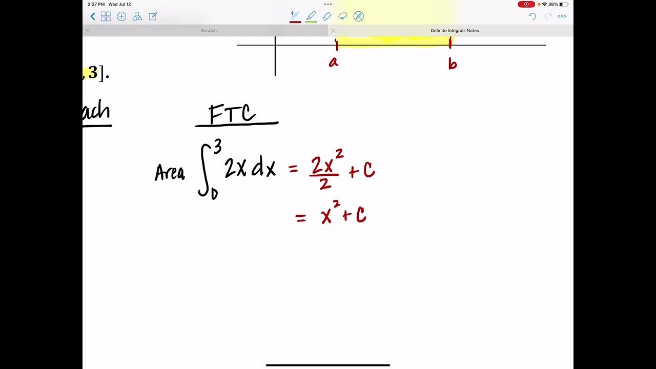
- 📉 The fundamental theorem of calculus is highlighted, stating that the integral's value depends only on the differential form's value at the endpoints of the path.
- 📈 The video contrasts the new interpretation of integrals with the traditional area-under-curve approach, showing how both methods yield the same result.
- 📝 An example of a path integral in the 2D plane and a single-variable integral are provided to demonstrate the differential form interpretation.
- 📐 The video explains how to compute integrals using differential forms by finding the antiderivative of the differential form and applying the fundamental theorem of calculus.
- 📉 The scalar field and covector field are visualized geometrically, showing how the path's intersection with the covector field's level sets can be counted to find the integral's value.
- 🌐 The video demonstrates changing coordinates and how it affects the appearance of the integral's expression but not the underlying geometry or the result.
- 🔄 The invariance of covector fields to the choice of coordinates is emphasized, pointing out that while the components of the field may change with different variables, the field itself remains the same.
- 📊 The video concludes by reiterating that covector fields are geometric objects that do not depend on the coordinate system used, which is why changing variables in an integral does not affect the final result.
Q & A
What is the main concept discussed in the video?
-The main concept discussed in the video is the differential form interpretation of integrals, which involves the idea of a path and a covector field in the computation of integrals.
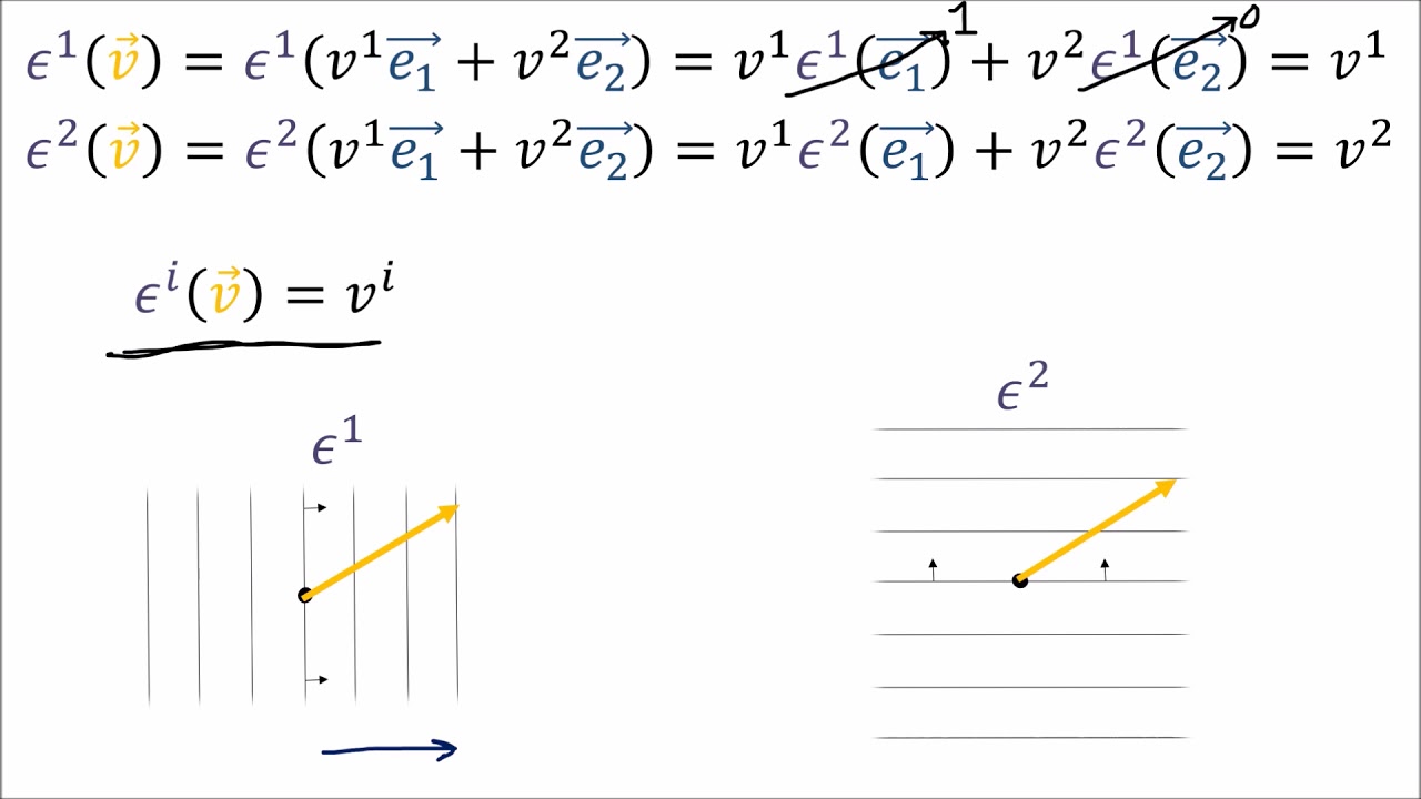
What is a covector field in the context of integrals?
-A covector field, also known as a differential form, is a set of contour curves that is used in the differential form interpretation of integrals to determine the value of the integral based on how many times a path intersects these curves.
How does the orientation of a path affect the computation of the integral?
-The orientation of a path affects the computation of the integral by adding plus 1 when the direction of the path is aligned with the covector orientation and minus 1 when it is aligned in the opposite direction.
What does the fundamental theorem of calculus tell us about the value of an integral?
-The fundamental theorem of calculus tells us that the value of an integral only depends on the value of the function at the endpoints of the path and is independent of the specific path taken, as long as the endpoints are the same.
Can you provide an example of how to compute an integral using the old interpretation involving areas under curves?
-An example given in the script is computing the area between the line -6x + 4 and the x-axis between x = 0 and x = 2. This is done by finding the antiderivative, evaluating it at the endpoints, and then subtracting the results.
How is the differential form interpretation different from the old interpretation of integrals?
-The differential form interpretation focuses on the path and covector field, considering the number of times the path intersects the covector curves, rather than the area under a curve.
What is the significance of the function F in the differential form interpretation?
-The function F is significant because it represents the scalar field, and its differential, DF, represents the covector field. The integral can be computed by evaluating F at the endpoints of the path according to the fundamental theorem of calculus.
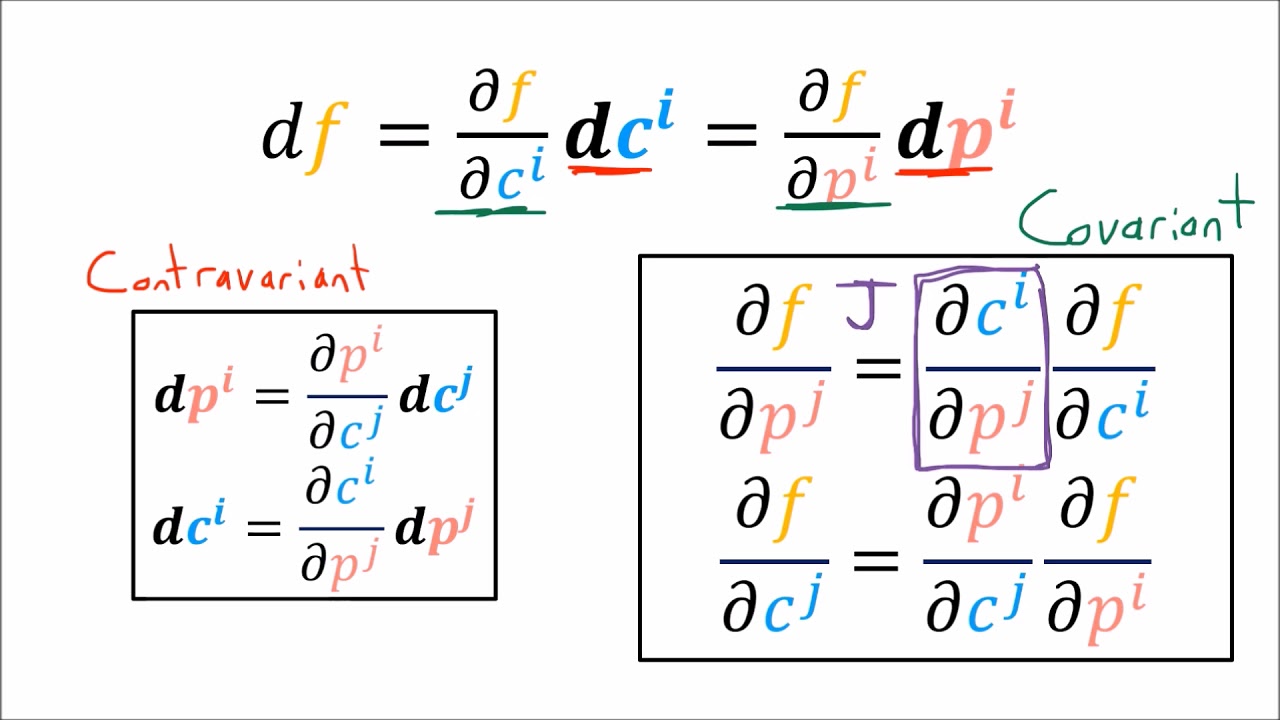
How does changing coordinates affect the computation of an integral?
-Changing coordinates affects the computation by altering the components of the covector field and the path equations, but the underlying geometry of the covector field and the path remains the same, ensuring the integral's result is invariant to the choice of coordinates.
Can you explain the process of changing variables in an integral and its effect on the result?
-Changing variables in an integral involves substituting the original variables with new ones, which changes the differentials and the path equations. Although the components of the covector field and the path may appear different, the result of the integral remains the same due to the invariance of the underlying geometric objects.
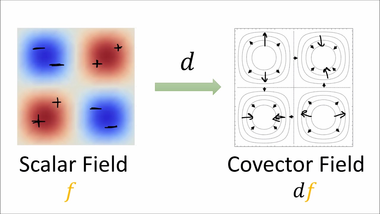
What is the geometric interpretation of the covector field DF?
-The geometric interpretation of the covector field DF is that it represents the level sets of the scalar field F, with arrows indicating the orientation towards positive values.
Why is the result of an integral the same regardless of the coordinate system used?
-The result of an integral is the same regardless of the coordinate system used because the covector field and the path are geometric objects that do not depend on the choice of coordinates. The components of the covector field may change with different coordinates, but the integral's result remains consistent.
Outlines
📚 Introduction to Differential Forms in Integration
This paragraph introduces the concept of differential forms in the context of integration. It explains that integrals involve a path and a covector field, emphasizing that the integral's value depends on the endpoints and not the path itself. The fundamental theorem of calculus is highlighted, showing that the integral's result is invariant to path choice. The paragraph sets the stage for comparing traditional area-under-curve interpretations with the new differential forms approach through examples.
🔍 Comparing Integration Interpretations with Examples
The second paragraph delves into comparing traditional single-variable integration with the differential forms approach through a specific example. It demonstrates how to compute an integral both by finding the area under a curve and by counting the number of covector field lines pierced by a path. The process involves rewriting the differential form as a derivative of a potential function, visualizing scalar and covector fields, and applying the fundamental theorem of calculus to find the integral's value, which remains consistent across methods.
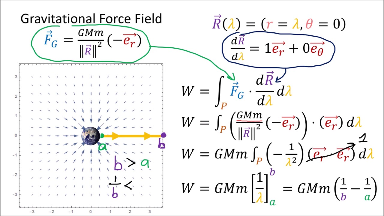
📈 Exploring Path Integrals in 2D with Parametric Paths
This paragraph extends the integration discussion to two-dimensional spaces, focusing on path integrals with parametric paths. It outlines the process of converting differentials into a single variable using a time parameter and then integrating over that parameter. The paragraph also introduces the differential form interpretation for this scenario, involving finding a scalar field that corresponds to the given differential form. The summary illustrates how to compute the integral both algebraically and geometrically, emphasizing the invariance of the integral's result to the choice of coordinates.
🌐 The Invariance of Differential Forms Across Coordinate Systems
The final paragraph discusses the geometric invariance of differential forms and paths across different coordinate systems. It uses examples to show how changing variables or applying a change of coordinates affects the components of the differential form but not the underlying geometry. The paragraph clarifies that while the components of a covector field depend on the choice of coordinates, the field itself remains invariant. This is analogous to how a vector's components change with different basis vectors but the vector itself remains the same. The summary reinforces the main point that the integral's outcome is consistent because it is based on geometric objects that are independent of coordinate systems.
Mindmap
Keywords
💡Integration
💡Differential Forms
💡Path Integral
💡Covector Field
💡Fundamental Theorem of Calculus
💡Scalar Field
💡Level Sets
💡Parametric Path
💡Change of Variables
💡Invariance
Highlights
Introduction to differential form interpretation of integrals involving a path and a covector field.
Explanation of how to compute integrals by counting the number of covector curves pierced by the path.
Clarification on the fundamental theorem of calculus and its geometric interpretation in integrals.
Comparison between the new interpretation of integrals and the traditional area-under-curve method.
Example of a path integral in the 2D plane and its computation using both old and new interpretations.
Demonstration of how to find a function F from its differential form DF/DX.
Visualization of F as a scalar field and its level sets as a covector field.
Explanation of the scalar field F and its independence from the choice of constant C.
Illustration of how the path integral is computed using the differential form interpretation.
Comparison of the results from the new interpretation with the traditional method for a 2D path integral.
Introduction of a second integral example involving both x and y variables in a 2D plane.
Process of expanding differentials DX and DY in terms of a parameter T for a parametrized path.
Conversion of a sum of covector fields into a single covector field using partial derivatives.
Identification of a function F that satisfies the conditions for the covector field components.
Demonstration of the scalar field F and its level sets for the covector field in a 2D integral.
Explanation of the invariance of covector fields to the choice of coordinate systems.
Illustration of changing coordinates and the effect on the appearance of the integral but not its underlying geometry.
Final summary emphasizing the geometric nature of covector fields and their independence from coordinate systems.
Transcripts
Browse More Related Video
Tensor Calculus 9: Integration with Differential Forms
Tensor Calculus 6: Differential Forms are Covectors
Tensors for Beginners 5: Covector Components (Contains diagram error; see description)
Tensor Calculus 8: Covector Field Transformation Rules (Covariance)
Definite Integrals

Switching bounds of definite integral | AP Calculus AB | Khan Academy
5.0 / 5 (0 votes)
Thanks for rating: