StatQuest: Principal Component Analysis (PCA), Step-by-Step
TLDRThis StatQuest episode with Josh Starmer demystifies Principal Component Analysis (PCA) through Singular Value Decomposition (SVD). It explains PCA's purpose, process, and application in data analysis, using a simple dataset of gene transcription in mice. The episode guides viewers through creating a PCA plot, identifying key variables, and understanding the value of each principal component in capturing data variation. It also introduces concepts like eigenvectors, eigenvalues, and scree plots, illustrating how PCA simplifies high-dimensional data into a comprehensible 2D representation.
Takeaways
- 📚 Principal Component Analysis (PCA) is a technique used to reduce the dimensionality of data while preserving as much variance as possible.
- 🔍 PCA uses Singular Value Decomposition (SVD) to break down data into principal components to find patterns and relationships within the data.
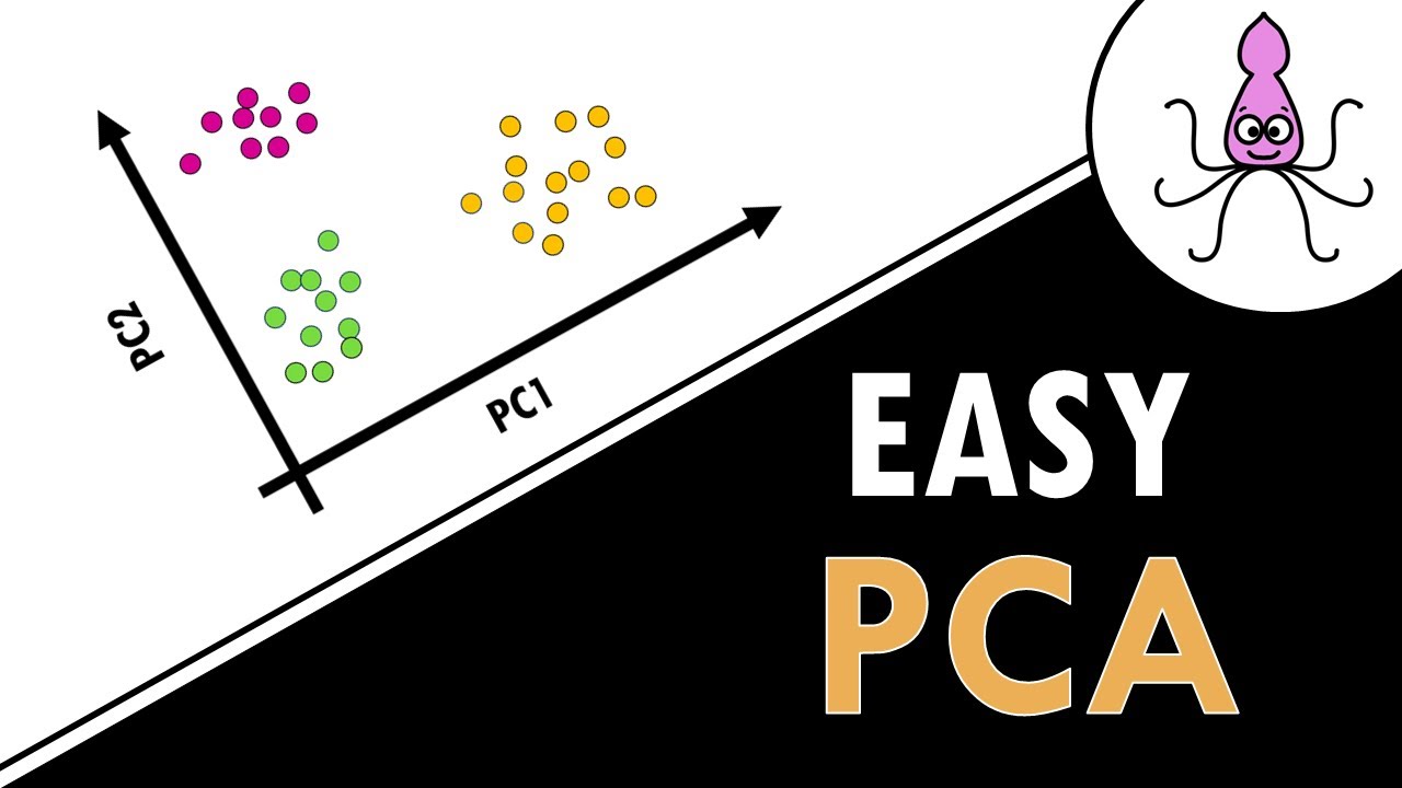
- 🐭 The script starts with a simple dataset of gene transcription in mice to illustrate the concept of PCA, with genes as variables and mice as samples.
- 📈 In a two-dimensional dataset, PCA projects data onto a line that maximizes the variance, creating the first principal component (PC1).
- 📉 The second principal component (PC2) is orthogonal to PC1 and captures the remaining variance, with each subsequent PC being orthogonal to the previous ones.
- 📝 PCA calculates the average measurement for each gene to find the center of the data, which is essential for shifting the data for analysis.
- 📊 The principal components are determined by maximizing the sum of squared distances from the projected points to the origin, rather than minimizing the distance to the line itself.
- 🍹 The 'recipe' for each principal component is a linear combination of the original variables, with the ratio indicating the importance of each variable in describing the data spread.
- 📏 The length of the vector representing a principal component is scaled to 1 in SVD, which helps in understanding the contribution of each variable.
- 📊 The script introduces the concept of eigenvectors and eigenvalues in the context of PCA, with eigenvectors showing the direction of the principal components and eigenvalues indicating the amount of variance explained.
- 📈 A scree plot is used to visualize the proportion of variance explained by each principal component, helping to decide how many components to retain for analysis.
- 🧩 Even with more complex datasets involving more variables, PCA follows the same principles, and the number of principal components is typically the minimum of the number of variables or samples.
Q & A
What is the main topic of the video script?
-The main topic of the video script is Principal Component Analysis (PCA) and how it is performed using Singular Value Decomposition (SVD).
What is the purpose of PCA?
-The purpose of PCA is to reduce the dimensionality of a data set while preserving as much of the variation in the data as possible, allowing for deeper insights into the data.
How is PCA related to the concept of genes and mice in the script?
-The script uses genes and mice as an example to explain PCA, where genes represent variables and mice represent individual samples in the data set.
What is the significance of the term 'loading scores' in PCA?
-Loading scores in PCA represent the proportions of each variable (e.g., Gene 1, Gene 2) in the linear combination that defines a principal component.
What does the term 'Eigenvector' refer to in the context of PCA?
-In PCA, the term 'Eigenvector' refers to the vector that defines the direction of a principal component, which is a linear combination of the original variables.
What is the role of the 'Eigenvalue' in PCA?
-The 'Eigenvalue' in PCA represents the amount of variance captured by the corresponding principal component.
What is the meaning of 'Singular Value' in the PCA process?
-The 'Singular Value' in PCA is the square root of the Eigenvalue and represents the magnitude of the principal component.
How does PCA decide if a fit is good or not?
-PCA decides if a fit is good by maximizing the sum of the squared distances from the projected points to the origin, which indicates how well the principal component captures the variation in the data.
What is the practical limit on the number of principal components in PCA?
-In practice, the number of principal components is limited to the number of variables or the number of samples, whichever is smaller.
What is a 'scree plot' and what does it represent?
-A 'scree plot' is a graphical representation that shows the proportion of variance accounted for by each principal component, helping to determine which components are most significant.
How can PCA with SVD be used to create a 2D plot from a higher-dimensional data set?
-PCA with SVD can create a 2D plot by projecting the data onto the first two principal components that account for the majority of the variation in the data set, thus simplifying the visualization.
Outlines
🧬 Introduction to Principal Component Analysis (PCA)
Josh Starmer introduces the concept of Principal Component Analysis (PCA) using Singular Value Decomposition (SVD). He explains the purpose of PCA, which is to simplify complex datasets with multiple dimensions into a lower-dimensional representation for easier analysis. The video begins with a simple dataset involving the transcription of two genes in six mice, using this as a basis to explain how PCA can cluster similar samples together and identify the most valuable variables for this clustering. The explanation includes a step-by-step guide on plotting data, centering it, and then using PCA to create a 2D PCA plot that maintains the relative positions of the data points.
📊 Understanding PCA's Line Fitting and Distance Metrics
This paragraph delves into how PCA evaluates the fit of a line to the data. It discusses two methods: minimizing the distances from the data points to the line or maximizing the distances from the projected points to the origin. The explanation uses the Pythagorean theorem to illustrate the inverse relationship between these distances. The paragraph emphasizes that PCA seeks to maximize the sum of squared distances from the projected points to the origin, which is referred to as the sum of squared distances (SS distances). The process involves rotating the line to achieve the best fit and calculating the Principal Component 1 (PC1), which is the line that maximizes this sum.
🔍 The Role of Gene Ratios and Linear Combinations in PCA
The script explains the importance of the ratio of Gene 1 to Gene 2 in describing data spread and introduces the term 'linear combination' used in mathematics to describe such ratios. The example provided calculates the length of the vector representing the first principal component and discusses how this vector is scaled to become a unit vector in the context of PCA with Singular Value Decomposition (SVD). The paragraph also introduces key PCA terminology, including 'Singular Vector', 'Eigenvector', 'loading scores', 'Eigenvalue', and 'Singular Value', providing a clear understanding of their roles in PCA.
📈 Deriving Additional Principal Components and Interpreting Variation
The paragraph continues the explanation of PCA by discussing how to derive additional principal components, such as PC2 and PC3, in a dataset with more variables. It emphasizes that these components are found by maximizing the sum of squared distances from the projected points to the origin, subject to the constraints of going through the origin and being perpendicular to existing components. The paragraph also explains how eigenvalues can be used to measure the amount of variation each principal component accounts for, introducing the concept of a scree plot as a graphical representation of these percentages.
🌐 Applying PCA to Higher Dimensional Data and Creating 2D PCA Plots
The final paragraph addresses how PCA can be applied to datasets with more than three variables, such as four genes per mouse, despite the inability to visualize higher-dimensional data. It explains that even without a visual representation, the mathematical process of PCA remains valid, and the resulting principal components can be used to create informative 2D PCA plots. The paragraph illustrates how to project samples onto the first two principal components, interpret the scree plot to determine the accuracy of the 2D representation, and ultimately create a 2D PCA plot that simplifies the data for easier analysis and visualization.
Mindmap
Keywords
💡Principal Component Analysis (PCA)
💡Singular Value Decomposition (SVD)
💡Gene Transcription
💡Data Centering
💡Principal Component (PC)
💡Eigenvector
💡Eigenvalue
💡Loading Scores
💡Scree Plot
💡Variation
💡Projection
Highlights
Introduction to Principal Component Analysis (PCA) using Singular Value Decomposition (SVD).
PCA's purpose is to provide deeper insights into data through dimensionality reduction.
Explanation of how PCA can be applied to a simple dataset of two genes in six mice.
Analogy of mice and genes to other scenarios like students and test scores, or businesses and market metrics.
Demonstration of how data can be plotted on a number line for a single gene measurement.
Visualization of data on a two-dimensional graph with two gene measurements.
Concept of adding dimensions for more genes, leading to the necessity of PCA for higher dimensions.
PCA's ability to create a 2D plot from multidimensional data and identify valuable variables for clustering.
Process of calculating the average measurements for Gene 1 and Gene 2 to find the data's center.
Shifting the data to have the center on the origin without changing relative positions.
Fitting a line to the data by maximizing the sum of squared distances from projected points to the origin.
Explanation of the Pythagorean theorem in the context of PCA to understand the relationship between distances.
Calculation of Principal Component 1 (PC1) as the best fitting line through the origin.
Interpretation of the slope of PC1 in terms of the importance of Gene 1 and Gene 2 in data spread.
Introduction to terminology: linear combination, singular vector, eigenvector, loading scores, eigenvalue, and singular value.
Process of determining Principal Component 2 (PC2) perpendicular to PC1 in a two-dimensional space.
Description of the scree plot as a graphical representation of the percentage of variation explained by each PC.
PCA application with three variables, emphasizing the method's scalability to more complex datasets.
Calculation of the proportion of variation explained by each PC and the use of a scree plot for visualization.
Transformation of a 3D graph into a 2D PCA graph using the first two principal components.
Discussion on the accuracy of PCA plots and the importance of considering additional PCs if they contribute significantly to variation.
Final summary of the PCA process, from understanding the data in a complex space to visualizing it in a simplified 2D plot.
Transcripts


5.0 / 5 (0 votes)
Thanks for rating: